1. Introduction

The purpose of this note is to provide an introduction to the Generalized Linear Model and a matricial formulation of statistical learning derived from the class of exponential distributions with dispersion parameter. We assume that the reader is comfortable with linear algebra and multivariable calculus, has an understanding of basic probability theory and is familiar with supervised learning concepts.

A number of regression and classification models commonly used in supervised learning settings turn out to be specific cases derived from the family of exponential distributions. This note is organized as follows:

1. Section 2 describes the family of exponential distributions and their associated Generalized Linear Model. The family described in [3] counts a significant number of distributions including e.g., the univariate Gaussian, Bernoulli, Poisson, Geometric, and Multinomial cases. Other distributions such as the multivariate Gaussian lend themselves to a natural generalization of this model. In order to do so, we extend the family of exponential distributions with dispersion parameter [3] to include symmetric positive definite dispersion matrices.
2. Section 3 derives the Generalized Linear Model Cost Function and its corresponding Gradient and Hessian all expressed in component form. We derive the expressions associated with the general case that includes a dispersion matrix. We also derive simplified versions for the specific case when the dispersion matrix is a positive scalar multiple of the identity matrix.
3. In Section 4, we limit ourselves to distributions whose dispersion matrix is a positive scalar multiple of the identity matrix. These are precisely the ones described in [3]. We express their associated Cost Function, Gradient and Hessian using concise matrix notation. We will separately analyze the case of the multivariate Gaussian distribution and derive its associated Cost Function and Gradient in matrix form in section 7.
4. Section 5 provides a matricial formulation of three numerical algorithms that can be used to minimize the Cost Function. They include the Batch Gradient Descent (BGD), Stochastic Gradient Descent (SGD) and Newton Raphson (NR) methods.
5. Section 6 applies the matricial formulation to a select set of exponential distributions whose dispersion matrix is a positive scalar multiple of the identity. In particular, we consider the following:
   • Univariate Gaussian distribution (which yields linear regression).
   • Bernoulli distribution (which yields logistic regression).
   • Poisson distribution.
   • Geometric distribution.
   • Multinomial distribution (which yields softmax regression).
6. Section 7 treats the case of the multivariate Gaussian distribution. It is an example of an exponential distribution with dispersion matrix that is not necessarily a positive scalar multiple of the identity matrix. In this case, the dispersion matrix turns out to be the precision matrix which is the inverse of the covariance matrix. We derive the corresponding Cost Function in component form and also express it using matrix notation. We then derive the Cost function’s Gradient, express it in matrix notation and show how to to minimize the Cost Function using BGD. We finally consider the specific case of a non-weighted Cost Function without regularization and derive a closed-form solution for the optimal values of its minimizing parameters.
7. Section 8 provides a python script that implements the Generalized Linear Model Supervised Learning class using the matrix notation. We limit ourselves to cases where the dispersion matrix is a positive scalar multiple of the identity matrix. The code provided is meant for educational purposes and we recommend relying on existing and tested packages (e.g., scikit-learn) to run specific predictive models.

2. Generalized Linear Model

Discriminative supervised learning models: Loosely speaking, a supervised learning model is an algorithm that when fed a training set (i.e., a set of inputs and their corresponding outputs) derives an optimal function that can make “good” output predictions when given new, previously unseen inputs.

More formally, let an denote the input and output spaces respectively. Let

x

denote a given training set for a finite positive integer The supervised learning algorithm will output a function that optimizes a certain performance metric usually expressed in the form of a Cost Function. The function can then be applied to an input to predict its corresponding output . Whenever is limited to a discrete set of values, we refer to the learning problem as a classification. Otherwise, we call it a regression.

The exercise of conducting predictions in a deterministic world is futile. Inject that world with a dose of randomness and that exercise becomes worthwhile. In order to model randomness, we usually lean on probabilistic descriptions of the distribution of relevant variables. More specifically, we may assume certain distributions on the set of inputs, the set of outputs, or joint distributions on inputs and outputs taken together. For the purpose of this note, we limit ourselves to models that make assumptions on the distribution of the output given the input, without giving any consideration to the underlying distribution of the inputs themselves. Such models are referred to as discriminative learning models.

Generalized Linear model: In essence, a Generalized Linear Model consists of three elements.

#1: A random component modeled as an instance from a family of probability distributions of the form:

(1)  

Modulo variables and maps naming, this family of distributions corresponds to the one introduced in [3]. It is defined for positive dispersion parameters We now introduce a more general version where the dispersion parameter could be a symmetric positive definite matrix . We define the enlarged family of exponential distributions to include those of the following form:

(2)  

where we define to be equal to The maps and parameters appearing in the expression above are described as follows:

• is known as the natural parameter vector. We will soon impose a relationship between the input and which will link the input to the output
• is a symmetric element of (i.e., a symmetric positive-definite matrix). We refer to it as the dispersion parameter matrix.
• is known as the non-negative base measure. It maps to the positive scalar value
• is a sufficient statistic of and has the same dimension as For all practical purposes, this means that the probability of a random variable taking on a particular value when conditioned on is equal to the probability of it taking the same value when conditioned on In other terms, whatever can be learned by conditioning on can also be learned by conditioning on
• is known as the log-partition function. It maps to where is a vector-valued map from into that depends only on We denote the components of the column vector by where each is a map from into

  The rationale for the log-partition nomenclature stems from it being chosen to ensure that integrates to 1. Doing so allows us to express as a function of the other parameters:

  

  

  

  

  (3)  

  In what follows, we derive expressions for the log-partition function’s Gradient and Hessian

  The log-partition function’s Gradient: We start by defining the one-form Gradient of with respect to to be the quantity:

  

  In Euclidean space, the associated column vector Gradient is denoted by we can write:

  

  

  

  

  As a result, we conclude that:

  (4)  

  The log-partition function’s Hessian: We first compute the second derivative of with respect to the vector as follows:

  

  

  

  

  

  

  

  

  

  We conclude that:

  (5)  

  An important implication is that the Hessian of with respect to is a covariance matrix and is hence symmetric positive semi-definite. This demonstrates that is convex in . Furthermore, is clearly linear in since As a result, is also convex in .

#2: A mean function that maps to the expected value of the sufficient statistic

(6)  

We can express the mean function in terms of the log-partition function or equivalently in terms of the map To do so, we first define the derivative operator of the vector-valued map with respect to to be the quantity:

Equations and show that:

(7)  

We could also invoke the chain rule and write:

It follows that:

(8)  

And hence, that:

(9)  

#3: A design criteria that imposes a linear relationship between the natural parameter vector and the input Note that the linearity condition is a matter of choice and one could theoretically investigate non-linear choices including e.g., quadratic or higher order relationships. The linearity condition is expressed as where:

• 
• is the design vector given by The are the features (i.e., components of the design vector) and the leading 1 accounts for the intercept term.
• is the coefficient matrix Note that reduces to a row vector whenever

The design criteria establishes a link between input and output. In other terms, knowledge of and the mean function allow one to compute:

Subsequently, one can make informed predictions about the output given a certain input as we will later see in sections 6 and 7.

The special case of a dispersion parameter: In what follows, we consider the special case of a dispersion matrix equal to a positive scalar multiple of the identity matrix We write . This case includes many of the known probability distributions including the univariate Gaussian, Bernoulli, Poisson, Geometric and Multinomial cases that we will revisit in section 6. As expected, this particular case lends itself to further simplification of the mean and the log-partition functions, as well as the latter’s Gradient and Hessian expressions:

• First, note that in this case, the form of the distribution reduces to:

  (10)  

  By defining to be the map taking to we can rewrite the probability distribution as:

  (11)  

  It becomes clear that the log-partition function can be expressed as:

  (12)  

• The Gradient of the log-partition function can also be simplified and written as:

  (13)  

  Equation coupled with equation demonstrate that:

  (14)  

  A noteworthy observation is that in this case, the mean function does not depend on the dispersion parameter It is completely determined by the natural parameter

• Lastly, note that equation shows that:

  (15)  

  Coupled with equation equation allows us to conclude that:

  (16)  

  An important implication is that the Hessian of with respect to is a positive multiple of a covariance matrix and is hence positive semi-definite. This shows that is convex in

3. Generalized Linear Model Cost Function, Gradient and Hessian

The long form basic Cost Function: In order to compute and conduct predictions on a given input one first needs to decide on the dispersion matrix and the matrix of coefficients. The performance of the predictive model will be dictated by the choice of and In our supervised learning setting, these two matrices will be jointly determined by:

• The pre-defined training set for a given integer
• The choice of an objective function to optimize. We refer to it as the Cost Function, denote it by and define it as a map that takes and as inputs and that outputs a real number. For the purpose of this note, we derive by applying the principle of Maximum Likelihood which we describe next.

Define the likelihood function associated with a training set to be

Our objective is to find the matrices and that maximize To proceed further, we assume that depends only on We get:

The presence of products coupled with the exponential nature of the conditional probability distribution makes it more appealing to invoke the natural logarithm function. Most importantly, the logarithm function is increasing on the subset of positive real numbers. This implies that maximizing the likelihood function is equivalent to maximizing the log-likelihood function over all possible choices of and We write:

Finally, note that maximizing is equivalent to minimizing We thus define the long form basic Cost Function to be the function:

that maps to:

(17)  

We use the descriptor long form to distinguish it from a shorter form associated with the special case of a dispersion matrix equal to a scalar multiple of the identity matrix. On the other hand, the basic attribute will be contrasted with a more general counterpart that will incorporate weights and a regularization parameter as we will see shortly.

The optimal values and must satisfy:

The long form general Cost Function: We can generalize further the Cost Function by accounting for two additional factors:

1. At times, when conducting a prediction on an input one might want to give more weight to training set points that are in the vicinity of One common way of doing so is by invoking a particular weight function defined as follows:

   

   

   Given an input on which a prediction needs to be conducted, one can evaluate at the different training points We let denote the quantity and refer to it as the weight attributed to the training point associated with input

   Different values of yield different weights attributed to the same training point. Moreover, larger values of the bandwidth paramter result in more inputs in the neighborhood of being attributed higher weights. In the extreme case when all training set inputs get a weight of

2. It is common practice in convex optimization to introduce a regularization component to the objective function. The purpose of it is to penalize high values of the optimization variables. In our case, the optimization variables consist of:
   • The coefficients matrix where

     

   • The dispersion matrix where

     

   The regularization term is usually proportional to the size of the variable, where size is measured according to some norm (e.g., L2 or L1). In our case, we add a regularization term given by The variable is the proportionality constant and the other factor is the sum of the squares of the L2 norm of each and each

Given a specific and we denote the corresponding long form general Cost Function by The subscripts are meant to highlight the potential dependence on weights (as dictated by the input ) and on the regularization parameter We have:

(18)  

An important observation is that is convex in To see why, recall from section 2 that the map is convex in Furthermore, is linear in and so is convex in . Moreover, is linear in and thus convex. Finally, one can easily show that is also convex in Being a positively scaled sum of convex functions, is thus convex in This in turn implies the existence of a globally minimizing value

In addition, note that all the terms appearing in are convex in (recall that we’ve seen in section 2 that the log-partition function is convex in except possibly for the term If is convex in then so will and as a result, so will This would then imply the existence of a globally minimizing

The long form general Cost Function’s Gradient: We define the Gradient of with respect to matrices and to be the map:

(19)  

where, and are defined as follows:

and

Note that and are taken to be one-forms (being covariant derivatives of the scalar function in the directions of vector and respectively). We subsequently represent them in Euclidean space as row vectors.

and the component of is:

Recall that by design, we chose and so As a result, the only value of for which contains the term is We simplify to obtain:

And hence conclude that:

(20)  

Similarly, one finds that the component of is:

(21)  

The long form general Cost Function’s Hessian: Let be the column vector whose components are given by:

We define the Hessian of the Cost Function with respect to matrices and to be the map:

We consider three cases:

• the component of is:

  

  

  

  Let and the map that takes to The chain rule allows us to write:

  

  

  Since we get whenever As a result:

  

  We conclude that:

  (22)  

• the component of is:

  

  

  We get:

  (23)  

• the and components of are equal and are given by:

  

  

  We get:

  (24)  

The short form basic Cost Function: With the exception of the multivariate Gaussian distribution, all the other probability distributions that we consider in this note have a dispersion matrix that is a positive scalar multiple of the identity matrix. For this particular case, equations and in section 2 showed that:

• The log partition function is given by where is now a positive scalar and is the natural parameter vector.
• The mean function is independent of the dispersion parameter and depends solely on the natural parameter We write for a given coefficient matrix and input vector

In what follows, we simplify the expression of the Cost Function associated with such a case and derive simpler formulae for the components of its Gradient and its Hessian. By substituting the matrix with (where and in equation and by applying equation we can write:

Minimizing with respect to is equivalent to minimizing the following quantity with respect to :

And since is a positive scalar, the optimal value of that minimizes this quantity is the same as the one that minimizes the following quantity:

(25)  

We refer to as the short form basic Cost Function. An important observation is that depends exclusively on And since in this particular case the mean function also depends only on one can find the optimal coefficient matrix by minimizing and then plugging it into to conduct predictions.

Equally important is the fact that is convex in The proof is similar to the one we previously used to establish the convexity of in

The short form general Cost Function: The same approach used to derive the long form general Cost Function from its basic counterpart can be applied to obtain the following short form general Cost Function:

Given a specific and the corresponding short form general Cost Function is the map that takes to:

(26)  

The short form general Cost Function’s Gradient: We define the Gradient of with respect to the matrix to be the map:

and the component of is:

Recall that by design, we chose and so As a result, the only value of for which contains the term is This allows us to write

And hence conclude that:

(27)  

The short form general Cost Function’s Hessian: We define the Hessian of with respect to the matrix to be the map:

where the block matrix is:

and the components of are:

Let and be the function mapping to The chain rule allows us to write:

Since we conclude that:

(28)  

4. Matricial formulation of the Cost Function, its Gradient, and its Hessian

In this section, we limit ourselves to the short form general Cost Function Since there is no room for confusion, we will drop the superscript refer to it simply as the Cost Function and denote it by In order to derive a concise notation for its Gradient , and its Hessian we first introduce relevant vectorial and matricial quantities. In what follows, we recall that denotes the dimension of the sufficient statistic denotes that of , denotes the number of input features and denotes the number of training examples.

• The coefficient matrix  is given by:

     

• The design matrix  is given by:

     

• The target matrix  for some is given by:

     

• The sufficient statistic matrix  is given by:

     

• The weight matrix  associated with input and weight function is given by:

     

• The regularization matrix  associated with parameter is given by:

     

• The log-partition vector  associated with the log-partition function that maps to is given by:

     

• The log-partition Gradient matrix  is given by:

     

• The second order diagonal matrix  where is given by:

     

• The unit vector  is given by:

     

The Cost Function in matrix form: Let and denote the row of and the column of If we have that then, one can easily see that

Substituting and with matrices and respectively, one concludes that the diagonal elements of are where Furthermore, multiplying this matricial product by the diagonal weight matrix one can see that the diagonal elements of the product are given by

As a result, we can rewrite equation more concisely in matrix form as:

(29)  

The Gradient of the Cost Function in matrix form: Using the same observation made in the previous paragraph regarding the product of three matrices, one can rewrite equation in a more concise matrix notation as follows:

(30)  

The Hessian of the Cost Function in matrix form: Similary, we can rewrite equation in matrix notation as follows:

(31)  

5. Algorithms to minimize the convex Cost Function

In this section too, we limit ourselves to the short form general Cost Function Our objective is to find the optimal If the weight functions are independent of for all training examples then will not depend on and once it is computed for a given input, it can be stored and used for all other inputs. This is known as a parametric setting. If the weight functions depend on then each will have a different associated with it. This procedure is known as non-parametric and is clearly computationally more demanding than its parametric counterpart. In what follows, we introduce three numerical methods for finding

1. Batch Gradient Descent (BGD): Suppose is a differentiable convex function of one variable. Starting at any one can get If its negative (positive), then at the function is decreasing (increasing). As a result, to get closer to the value of that minimizes one can try a value ().

   One way of updating the value of is by letting for some positive learning rate This procedure can be repeated until convergence. Note however, that the choice of is critical since too large a value will cause divergence, while a value that is too small will cause slow convergence.

   

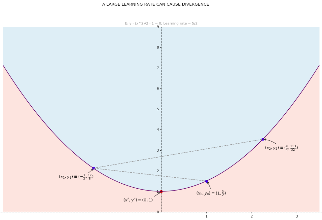
   The same can be said of differentiable functions of variables () where this logic gets applied to each variable. In this context, we replace with the Gradient of and the learning rate with the learning rate matrix defined as:

      

   One can estimate the optimal matrix by running the following algorithm known as Batch Gradient Descent (BGD). We let iter denote an iteration count variable and max-iter denote the maximum number of allowed iterations before testing for convergence:

   
   (It could be initialized to e.g., the zero by matrix).

   For (iter  max-iter)

   

   

   

   Update all the -dependent quantities including

   

   

   

   

   

   So the following update is performed:

   
   

   

   where we have:

   

   and where

   Note that BGD requires that all the entries of the new coefficient matrix be simultaneously updated before they can be used in the next iteration.

2. Stochastic Gradient Descent (SGD):In BGD, everytime we updated the value of we had to perform a summation over all training examples as mandated by . In SGD, we drop the summation to achieve faster updates of the coefficients. In other terms, for each training example and SGD conducts the following update round:

      

   The entries of the new coefficient matrix must get simultaneously updated for each training example in each iteration before they can be used in the next instance. SGD usually achieves acceptable convergence faster than BGD, especially when the size of the training set is very large

   In order to describe the SGD algorithm in a more concise matrix form, we define a set of new matrices where and where the entry is given by:

   

   SGD is a variant of BGD that runs the following algorithm:

   
   (It could be initialized to e.g., the zero by matrix).

   For (iter  max-iter)

   

   For ()

   

   

   

   Update all the -dependent quantities including

   

   

   

   

   

   

3. Newton-Raphson (NR): The choice of the learning rate used in BGD and SGD is of special importance since it can either cause divergence or help achieve faster convergence. One limiting factor in the implementation of the previous Gradient descent algorithms is the fixed nature of . Computational complexity aside, it would be beneficial if at every iteration, the algorithm could dynamically choose an appropriate so as to reduce the number of steps needed to achieve convergence. Enters the Newton Raphson (NR) method.To motivate it, we lean on a Taylor series expansion of the Cost Function about a point (i.e., coefficient matrix) up to first order. We get:

   

   

   If we want to get to the optimal in one step, we need to set to when evaluated at and . Taking the first derivative with respect to of the right and left hand sides of the approximation, and noting that is a constant and are constants, we get:

   

   

   Setting to 0 for all i we get:

   

   

   Recall that and are both elements of We define the vectorized versions of and to be the elements of given by:

      

      

   We can subsequently write the above conditions in a more concise matrix form as follows:

   

   Which gives the following NR algorithm:

   
   (It could be initialized to e.g., the zero by matrix).

   For (iter  max-iter)

   

      

   

   

   Update all the -dependent quantities including

   

   

   

   

   

   

   

   Here too, the update rule is simultaneous. This means that we keep using until all entries have been calculated, at which point we update to

   NR is usually faster to converge when measured in terms of number of iterations. However, convergence depends on the invertibility of the Hessian at each iteration. This is not always guaranteed (e.g., multinomial classification with more than two classes). Alternatively, one could circumvent this problem by applying a modified version of NR as described in e.g., [2]. Furthermore, even when convergence is guaranteed, NR can be computationally taxing due to the matrix inversion operation at each iteration. Taking that into account, usage of NR is usually preferred whenever the dimensions of are small (i.e., small and

6. Specific distribution examples

In what follows, we consider a number of probability distributions whose dispersion matrix is of the form where is a positive dispersion scalar and is the identity matrix for In order to devise the relevant discriminative supervised learning model associated with an instance of the class of such distributions, we proceed as follows:

Step 1: Identify the dimensions of the target matrix where is the number of training examples and the dimension of each output.

Step 2: Identify the natural parameter and dispersion parameter associated with the exponential distribution, compute the sufficient statistic matrix compute the non-negative base measure and derive the log-partition function Identify the dimensions of the coefficient matrix

Step 3: Compute the set of functions

Step 4: If needed (e.g., in the case of NR algorithm), compute the set of functions

Step 5: Compute the log-partition vector

Step 6: Compute the log-partition Gradient matrix

Step 7: If needed (e.g., in the case of NR algorithm), compute the set of second order diagonal matrices

Step 8: Compute the Cost Function , its Gradient and its Hessian

Step 9: Calculate the optimal using e.g., BGD, SGD, NR or using a closed form solution if applicable.

Step 10: Test the model on an adequate test set and then conduct predictions on new input using the mean function that maps to

i. The univariate Gaussian distribution: The corresponding probability distribution is:

We rewrite it in an equivalent form that makes it easier to identify as a member of the exponential family:

Step 1: The target matrix In other terms, each training example has a univariate output associated with it.

Step 2: We identify the following quantities:

• The natural parameter
• The sufficient statistic Matrix (here,
• The dispersion matrix is
• The non-negative base measure is
• The log-partition function maps to:

  

• The coefficient matrix is a row vector

Step 3: The function is the identity map that takes to

Step 4: If needed (e.g., in the case of NR algorithm), the function maps to the constant value

Step 5: The log-partition vector is given by:

Step 6: The log-partition Gradient matrix is:

Step 7: If needed (e.g., in the case of NR algorithm), the second order diagonal matrix is the by identity matrix

Step 8: Compute the Cost Function , its Gradient and its Hessian

Step 9: Calculate the optimal using e.g., BGD, SGD, NR.

Step 10: Test the model on an adequate test set and then conduct predictions on new input using the mean function that maps to:

The supervised learning model associated with the univariate Gaussian distribution coincides with the familiar linear regression model when we consider the short form basic Cost Function . Recall that the basic form has no dependence on either the regularization parameter or the input In this case, the weight matrix is equal to and the regularization matrix is equal to

To see this equivalence, we rewrite equation as:

Minimizing over is equivalent to minimizing over We thus retrieve the familiar least-square model.

It also turns out that one can calculate the optimal coefficient matrix in closed form. Recalling that is convex in we can find by setting equal 0. Substituting with with with and with in equation we get:

Setting this Gradient to leads to the normal equation that allows us to solve for in closed form:

ii. The Bernoulli (Binomial) distribution: The corresponding probability distribution is:

where the outcome is an element of and where and We rewrite it in an equivalent form that makes it easier to identify as a member of the exponential family:

Step 1: The target matrix In other terms, each training example has a binary output associated with it.

Step 2: We identify the following quantities:

• The natural parameter (and so
• The sufficient statistic Matrix (here,
• The dispersion matrix is
• The non-negative base measure is
• The log-partition function maps to:

     

• The coefficient matrix is a row vector

Step 3: The function maps to

Step 4: If needed (e.g., in the case of NR algorithm), the function maps to

Step 6: The log-partition Gradient matrix is:

Step 7: If needed (e.g., in the case of NR algorithm), the second order diagonal matrix is given by:

Step 8: Compute the Cost Function , its Gradient and its Hessian

Step 9: Calculate the optimal using e.g., BGD, SGD, NR.

Step 10: Test the model on an adequate test set and then conduct predictions on new input using the mean function (also known as the sigmoid function) that maps to:

Note that:

Moreover, we know that:

As a result, we conclude that:

This is none else than the familiar logistic regression model where we predict whenever and otherwise. This classification highlights the presence of a decision boundary given by the set of inputs that satisfy This is justified by the fact that

iii. The Poisson distribution: The probability distribution with poisson rate is:

The outcome is usually a count of an event occurrence. We can rewrite the distribution in an equivalent form that makes it easier to identify as a member of the exponential family:

Step 1: The target matrix In other terms, each training example has a non-negative integer output associated with it.

Step 2: We identify the following quantities:

• The natural parameter (and so
• The sufficient statistic Matrix (here,
• The dispersion matrix is
• The non-negative base measure is
• The log-partition function maps to:

     

• The coefficient matrix is a row vector

Step 3: The function maps to

Step 4: If needed (e.g., in the case of NR algorithm), the function maps to

Step 5: The log-partition vector is given by:

Step 6: The log-partition Gradient matrix is:

Step 7: If needed (e.g., in the case of NR algorithm), The second order diagonal matrix is given by:

Step 8: Evaluate the Cost Function , Gradient and Hessian

Step 9: Calculate optimal using e.g., BGD, SGD, NR.

Step 10: Run the model on an adequate test set and then conduct predictions on new input using the mean function that maps to:

Note that the range of is although the sufficient statistic is in This is because the mean function outputs the expected value of the sufficient statistic. So one would still need to map the expected value outputed by to an integer in

iv. The Geometric distribution: The corresponding probability distribution is:

The outcome is The distribution calculates the probability of having a success after exactly trials, where the probability of success is equal to We rewrite it in an equivalent form that makes it easier to identify as a member of the exponential family:

Step 1: The target matrix In other terms, each training example has a positive integer output associated with it.

Step 2: We identify the following quantities:

• The natural parameter (and so
• The sufficient statistic Matrix
• The dispersion matrix is
• The non-negative base measure is
• The log-partition function maps to:

     

• The coefficient matrix is a row vector

Step 3: The map takes to

Step 4: In case required (e.g., in the case of NR algorithm), the function maps to

Step 5: Derive the log-partition vector:

Step 6: The log-partition Gradient matrix is:

Step 7: If needed (e.g., in the case of NR algorithm), the second order diagonal matrix is given by:

Step 8: Evaluate the Cost Function , Gradient and Hessian

Step 9: Evaluate the optimal using e.g., BGD, SGD, NR.

Step 10: Run the model on a test set and conduct predictions on new input using the mean function that maps to:

Note that the range of is although the sufficient statistic is in This is because the mean function outputs the expected value of the sufficient statistic. So one would still need to map the expected value outputed by to an integer in

v. The Multinomial distribution: The corresponding probability distribution is:

Here, is a function of that returns 1 if and only if and returns 0 otherwise. One can think of this distribution as the probability of taking a value in the set with:

…

We rewrite it in an equivalent form that makes it easier to identify as a member of the exponential family:

Step 1: The target matrix In other terms, each training example has an integer output associated with it.

Step 2: We identify the following quantities:

• The natural parameter is given by:

     

• The sufficient statistic of is:

     

  As a result, the sufficient statistic matrix is given by:

     

  Here,

• The dispersion matrix is
• The non-negative base measure is
• The log-partition function maps to:

     

• The coefficient matrix is given by:

     

Step 3: the function corresponds to the following mapping:

Step 4: If needed (e.g., in the case of NR algorithm), the function can be computed as follows:

where if and otherwise.

Step 5: We evaluate the log-partition vector to be:

Step 6: The log-partition Gradient matrix is given by:

Step 7: If needed (e.g., in the case of NR algorithm), the second order diagonal matrix is the diagonal matrix whose entry () is given by:

Step 8: Calculate the Cost Function , its Gradient and its Hessian

Step 9: Compute the optimal using e.g., BGD, SGD, NR.

Step 10: Test the model on a test set and then conduct predictions on new input using the mean function that maps to:

Note that by definition, we have Substituting the previously derived expression for we get:

Observing that

We get

This is the familiar softmax regression model. We predict whenever and where we define to be equal to This classification highlights the presence of decision boundaries that delimit distinct zones where the zone correspond to the set of vectors for which .

Note that logistic regression is a special case of softmax regression when

7. The multivariate Gaussian distribution case

The multivariate Gaussian distribution is given by:

where and is a symmetric positive definite matrix in

Note that the symmetry and positive definiteness of imply the symmetry and positive definiteness of as we now demonstrate.

• Proof that is symmetric: We claim that for any invertible matrix it holds that Indeed, letting denote the identity matrix, we have the following chain of equalities:

     

  It ensues that By virtue of being positive definite, is invertible and we get as a result that Invoking the symmetric nature of we then conclude that This shows that is symmetric.

• Proof that is positive definite: Being positive definite, exclusively admits positive eigenvalues. But the eigenvalues of are the reciprocals of those of and hence are also positive. This in turn implies that is positive definite.

We rewrite the probability distribution in an equivalent form that makes it easier to identify as a member of the exponential family with dispersion matrix:

Being a scalar, the quantity is equal to its transpose And since is symmetric, it must be that Moreover, the determinant of satisfies As a result, we write:

Step 1: The target matrix In other terms, each training example has a multivariate output associated with it.

Step 2: We identify the following quantities:

• The natural parameter vector
• The sufficient statistic Matrix Note that the dimension of the sufficient statistic is equal to the dimension of
• The dispersion matrix is which is not necessarily a positive multiple of the identity matrix The inverse of the covariance matrix is also usually known as the precision matrix.
• The non-negative base measure is:

  

• The log-partition function maps to:

     

  where is the map that takes to

  We can also compute the derivative of with respect to

     

• The coefficient matrix is

Step 3: We claim that the Gradient of with respect to is the map from to that takes to

To see why, note that if is a given matrix and maps vector to then

As a result,

And so:

We then conclude that:

Step 4: We now turn to computing the cost function derived from conducting maximum likelihood estimation using the multivariate Gaussian distribution. After substituting the relevant parameters in equation we get:

We rewrite this more concisely using matrix notation as follows:

(32)  

We have seen earlier that the long form general Cost Function is convex in Moreover, we showed that if is convex in then so will the Cost Function. We now demonstrate that for the case of the multivariate Gaussian, is indeed convex in To do so, we prove the equivalent claim that is convex in To see why, note that:

Note that the first term is linear in and hence convex in The last term is independent of The second term is a negative multiple of the natural logarithm of the determinant of a positive definite matrix. To establish the convexity of this quantity, we first find the Gradient of which turns out to be equal to (for a proof, the reader can refer to e.g., section 4.A.1 of [1]). We then compute the Hessian which turns out to be equal to This shows that the Hessian is positive definite which implies that is convex in

Step 5: We now turn to computing the Cost Function’s Gradient as specified by equation In order to do so, we first prove some identities involving the derivative of a Trace.

• Gradient of :

  In what follows, the quantity evaluates to 1 if and 0 otherwise. First of all, note that:

  

  

  and we can express the component of its derivative with respect to as follows:

     

  (since and are symmetric.)

  As a result, we conclude that:

  (33)  

  Similarly, we can follow the same procedure to find that:

  (34)  

• Gradient of :

  We first notice that:

  

  

  Since is symmetric, we can equivalently write this equality as:

     

  We then apply the same logic as before and demonstrate that:

  (35)  

  And that:

  (36)  

• Gradient of :

  Given the lack of dependency on it is obvious that:

  (37)  

  Furthermore, observing that is symmetric and applying the same methodology that we previously used allow us to readily show that:

  (38)  

• Gradient of :}

  Here too, independence of justifies that:

  (39)  

  On the other hand, we have:

     

  We stated earlier that (see e.g., section 4.A.1 of [1]). As a result, we conclude that:

  (40)  

• Gradient of and :}

  Clearly:

  (41)  

  Furthermore, we can apply the same calculation as before to conclude that:

  (42)  

  (43)  

The Gradient of the Cost Function can now be readily computed as:

(44)  

(45)  

Step 6: With the Cost function and its gradient thus derived, we can use numerical algorithms to find the optimal and that minimize In what follows we illustrate how this can be done using BGD. Recall that denotes the learning rate matrix that was previously introduced in section 5, iter is an iteration count variable and max-iter is the maximum number of allowed iterations before testing for convergence:

(They could be initialized to e.g.,  and  respectively).

For (iter  max-iter)

Update all the and -dependent quantities including:

It is important to note that the entries of matrices and must get simultaneously updated before they can be used in the next iteration.

Step 7 Test the model on an adequate test set and then conduct predictions on new input using the mean function that maps to:

It turns out that one can calculate the optimal coefficient matrix and the optimal dispersion matrix in closed form whenever the Cost Function is expressed in its long basic form . In other terms, whenever we assume that the weight matrix is independent of and equal to the identity matrix, and that the regularization matrix is independent of and equal to the 0 matrix. In this case, equation yields:

Recall that the Cost Function is convex in and in We can therefore find and by setting the Gradient with respect to and to to 0. By doing so, we get:

Since is positive definite, this is equivalent to We then retrieve the familiar normal equation we obtained in the univariate case:

Similarly, by setting we find:

8. Python implementation

This section provides a python script that implements the Generalized Linear Model Supervised Learning class using matrix notation. We limit ourselves to cases where the dispersion matrix is a positive scalar multiple of the identity matrix. We emphasize that the code is meant for educational purposes and we recommend using tested packages (e.g., Scikit-Learn) to run specific predictive models.

import sys;
import math;
import numpy as np;



# THE GLM CLASS DEFINES AN INSTANCE OF A PREDICTION PROBLEM. 
# IN ORDER TO DEFINE AN INSTANCE, ONE SHOULD PROVIDE THE FOLLOWING:
# -----------------------------------------------------------------------
# ------X_train (m by (n+1)): Training set input (including all-1 column)
# --------------------------- m is number of training examples and n is 
# --------------------------- number of features.
# -----------------------------------------------------------------------
# ------Y_train (m by r): Output matrix for the training set.
# --------------------------- m is number of training examples and r is
# --------------------------- the output's dimension.
# -----------------------------------------------------------------------
# ------reg_model: String defining the probability distribution to be
# --------------------------- used for regression / classification. We
# --------------------------- include the following (but can be expanded
# --------------------------- further): "normal", "binomial", "poisson", 
# --------------------------- "geometric", "multinomial".
# -----------------------------------------------------------------------
# ------p: Refers to the dimension of the sufficient stastic. For most
# --------------------------- examples used here, it is equal to 1. For
# --------------------------- multinomial classification it is equal to 
# --------------------------- one less than the number of classes.
# -----------------------------------------------------------------------
# ------regu_lambda: Refers to the regularization parameter lambda. it is
# --------------------------- a scalar that can be set to 0.
# -----------------------------------------------------------------------
# ------weight_flag: Should be set to 1 if one wishes to conduct weighted
# --------------------------- regression/ classification. It relies on
# --------------------------- the familiar bell-shaped function. In this 
# --------------------------- case, the data point where prediction is to
# --------------------------- be made defines the weights to be used. As
# --------------------------- a result, that specific data point must be
# --------------------------- included as an input to the fitting process
# --------------------------- as we later describe in the "fit" method.
# --------------------------- If no weights are needed, set flag to 0.
# -----------------------------------------------------------------------
# ------weight_tau: Holds the bandwidth value tau of the weight function.
# --------------------------- It is set to 1 by default and is only used
# --------------------------- when the weight_flag is set to 1.
# -----------------------------------------------------------------------

class Glm:
    def __init__(self, X_train, Y_train, reg_model, p, regu_lambda, 
                                            weight_flag, weight_tau = 1):                 
        self.X_train = X_train                     
        self.Y_train = Y_train                     
        self.reg_model = reg_model                 
        self.p = p
        self.regu_lambda = regu_lambda             
        self.weight_flag = weight_flag             
        self.weight_tau = weight_tau           


    def display_X_train(self):              
        print "\n The training set input matrix is:\n", self.X_train
        
        
    def display_Y_train(self):              
        print "\n The training set output is:\n", self.Y_train
        
        
    def display_reg_model(self):            
        print "\n The model is a: ", self.reg_model, " distribution"
        
        
    def display_regu_lambda(self):          
        print "\n The regularization parameter is: ", self.regu_lambda
        
        
    def display_weight_flag(self):          
        if (self.weight_flag == 1): 
            print "\n The current prediction instance is weighted"
            
        elif (self.weight_flag == 0): 
            print "\n The current prediction instance is not  weighted"
            
        else: print "\n Flag value not recognized. Please insert 1 or 0"
        
        
    def display_weight_tau(self):           
        if (self.weight_flag == 1): 
            print "\n The weight function bandwidth is ", self.weight_tau
        
        else: print "\n The current prediction is not weighted."
        

        
# THE GLM CLASS INCLUDES 3 GETTER METHODS. THESE ARE:
# ------get_m(): Returns total number of training examples.
# -----------------------------------------------------------------------
# ------get_n(): Returns total number of input features. We subtract 1 
# --------------------------- to exclude X_train's all-1 column.
# -----------------------------------------------------------------------
# ------get_p(): Returns dimension of the sufficient statistic.
# -----------------------------------------------------------------------
   
    def get_m(self):    
        return self.X_train.shape[0]
            
    def get_n(self):    
        return self.X_train.shape[1] - 1
                                                                                         
    def get_p(self):                                                                
        return self.p



# THE GLM CLASS LEVERAGES MATRIX NOTATION. THE FOLLOWING METHODS HELP 
# GENERATE THE RELEVANT MATRICIAL QUANTITIES.
# ------weight_bell_func(x, training_i): Returns the weight specific 
# --------------------------- to training example i, as dictated by input
# --------------------------- x (which is an (n+1) by 1 vector). The
# --------------------------- The weight we use is the bell-shaped one 
# --------------------------- with bandwidth tau.
# -----------------------------------------------------------------------
# ------generate_W(x): Generates the weight matrix W associated with
# --------------------------- input x. When the weighted regression flag
# --------------------------- is 0, it is the (m by m) identity matrix.
# -----------------------------------------------------------------------
# ------generate_L(): Generates the ((n+1) by (n+1)) regularization
# --------------------------- matrix L. It is equal to "lambda" times the
# --------------------------- ((n+1) by (n+1)) identity matrix.
# -----------------------------------------------------------------------
# ------generate_T(): Generates the (m by p) sufficient statistic matrix
# --------------------------- T. It depends on the probabilistic model.
# --------------------------- Note that for the multinomial model, we 
# --------------------------- label classes from 0 to (p-1).
# -----------------------------------------------------------------------
  
    def weight_bell_func(self, x, training_i):
        return math.exp(-np.dot((self.X_train[training_i,::] - x.T),
                                (self.X_train[training_i,::] - x.T).T)/
                                        float(2*(self.weight_tau**2)))


    def generate_W(self, x):                                    
        m = self.get_m()
        W = np.eye(m, dtype=np.float64)
                                 
        if (self.weight_flag == 1):
            for i in range(m): 
                W[i,i] = self.weight_bell_func(x, i)
            
        return W
    
    
    def generate_L(self):                                          
        n = self.get_n()
        L = self.regu_lambda * np.eye(n+1, dtype=np.float64)
        
        return L
    
    
    def generate_T(self):                                               
        p = self.get_p()
        m = self.get_m()
        T = np.zeros((m,p), dtype=np.float64)  
                               
        if (self.reg_model in ["normal", "binomial", "poisson", 
                                                            "geometric"]):
            T = self.Y_train
            
        elif (self.reg_model == "multinomial"): 
            for i in range(m):
                for j in range(p):
                    if(int(self.Y_train[i,0]) == j): 
                        T[i,j] = 1
                        
        else:
            print "No valid model has been inserted. System exiting now"
            sys.exit()
            
        return T
    

  
# TO GENERATE THE REMAINING RELEVANT MATRICES, THE GLM CLASS MAKES USE OF
# QUANTITIES BUILT OFF THE LOG-PARTITION FUNCTION AND ITS DERIVATIVES.
# THE LOG-PARTITION FUNCTION IS PROBABILITY DISTRIBUTION-DEPENDENT.
# ------a_func(eta): Returns the value of the relevant log-partition 
# --------------------------- function evaluated at eta. For most of the 
# --------------------------- encoded distributions, the first derivative
# --------------------------- is a function from R to R. For the case of
# --------------------------- the multinomial, it is a map from R^p to R.
# -----------------------------------------------------------------------
# ------a_first_deriv(eta, index): Returns the value of the partial
# --------------------------- derivative of the log-partition function
# --------------------------- with respect to the index's variable and
# --------------------------- evaluated at eta. For most of the encoded
# --------------------------- distributions, the first derivative is a 
# --------------------------- function from R to R. For the case of the
# --------------------------- multinomial, it is a map from R^p to R.
# -----------------------------------------------------------------------
# ------a_second_deriv(eta, index1, index2): Returns the value of the 2nd
# --------------------------- partial derivative of the log-partition
# --------------------------- function with respect to the 2 indexes'
# --------------------------- variables index1 and index2 evaluated at 
# --------------------------- eta. For most of the encoded distributions,
# --------------------------- the second derivative is a function from R 
# --------------------------- to R. For the case of the multinomial, it
# --------------------------- is a function from R^p to R.
# -----------------------------------------------------------------------
   
    def a_func(self, eta):                                              
        p = self.get_p()
        if (self.reg_model == "normal"):       
            return eta**2/float(2)
                                             
        elif (self.reg_model == "binomial"):
            return math.log(1+math.exp(eta))
                                   
        elif (self.reg_model == "poisson"):
            return math.exp(eta)
                                              
        elif (self.reg_model == "geometric"):
            return math.log(math.exp(eta)/float(1-math.exp(eta)))
              
        elif (self.reg_model == "multinomial"):
            val = 0
            
            for j in range(p): 
                val += math.exp(eta[j])
                                                                    
            return math.log(val + 1)
        
        else:
            print "No valid model has been inserted. System exiting now"
            sys.exit()
        
        
    def a_first_deriv(self, eta, index):
        p = self.get_p() 
        if (self.reg_model == "normal"):
            return eta
                                             
        elif (self.reg_model == "binomial"):
            return math.exp(eta)/float(1+math.exp(eta))
                   
        elif (self.reg_model == "poisson"):
            return math.exp(eta)
                                         
        elif (self.reg_model == "geometric"):
            return 1/float(1-math.exp(eta)) 
                             
        elif (self.reg_model == "multinomial"):
            denom = 1
            
            for j in range(p):
                denom += math.exp(eta[j])                                             
            
            return math.exp(eta[index])/float(denom) 
        
        else:
            print "No valid model has been inserted. System exiting now"
            sys.exit()
            
            
    def a_second_deriv(self, eta, index1, index2):
        p = self.get_p()          
        if (self.reg_model == "normal"):
            return 1              
                           
        elif (self.reg_model == "binomial"):
            return math.exp(eta)/float((1+math.exp(eta))**2)
            
        elif (self.reg_model == "poisson"):
            return math.exp(eta)        
                               
        elif (self.reg_model == "geometric"):
            return math.exp(eta)/float((1-math.exp(eta))**2)
         
        elif (self.reg_model == "multinomial"):
            denom = 1
            
            for j in range(p):
                denom += math.exp(eta[j])
                                                        
            val = -math.exp(eta[index1]+eta[index2])/float(denom**2)
            
            if (index1 == index2):
                val += math.exp(eta[index1])/float(denom)
                
            return val
        
        else:
            print "No valid model has been inserted. System exiting now"
            sys.exit()
  

  
# THE REMAINING RELEVANT MATRICES NEEDED TO COMPLETE THE OPTIMIZATION
# EXERCISE ARE GIVEN BELOW:
# ------generate_A(theta): Returns the (m by 1) vector whose entries 
# --------------------------- are relevant values of the log-partition
# --------------------------- function. "A" is theta-dependent.
# -----------------------------------------------------------------------
# ------generate_D(theta): Returns the "D" matrix. It is theta-dependent.
# -----------------------------------------------------------------------
# ------generate_S_uk(theta, u, k): Returns the S_uk block. It is used
# --------------------------- to compute the Cost Function's Hessian.
# -----------------------------------------------------------------------
          
    def generate_A(self, theta):
        m = self.get_m()
        A = np.zeros((m,1), dtype = np.float64)
        
        for i in range (m):
            A[i] = self.a_func(np.dot(self.X_train[i,::],theta.T).T)
        
        return A
    
    
    def generate_D(self, theta):
        p = self.get_p()
        m = self.get_m()
        D = np.zeros((p,m),dtype = np.float64)
        
        for i in range(p):
            for j in range(m):
                D[i,j]= self.a_first_deriv(
                            np.dot(self.X_train[j,::],theta.T).T, i)
            
        return D
    
    
    def generate_S_uk(self, theta, u, k):
        m = self.get_m()
        S_uk = np.zeros((m,m),dtype = np.float64)
        
        for i in range(m): 
            S_uk[i,i] = self.a_second_deriv(
                            np.dot(self.X_train[i,::],theta.T).T, u, k)            
        return S_uk;
    
    
        
# THE FOLLOWING METHODS COMPUTE THE COST FUNCTION, GRADIENT, AND HESSIAN.
# ------cost_Grad_Hess(self, theta, x): Takes theta and x as input, and 
# --------------------------- outputs 3 quantities: 
# --------------------------- 1) Cost Function evaluated at theta and x.
# --------------------------- 2) Gradient evaluated at theta and x.
# ---------------------------    (It is a p by (n+1) matrix)
# --------------------------- 3) Hessian at theta and x.
# ---------------------------    (It is a p*(n+1) by p*(n+1) matrix)
# -----------------------------------------------------------------------
# ------stoch_Grad(x, i, theta): Used in stochastic gradient descent. 
# --------------------------- Input i refers to the relevant training
# --------------------------- example while theta and x are as before.
# -----------------------------------------------------------------------

    def cost_Grad_Hess(self, theta, x):
        m = self.get_m()
        n = self.get_n()
        p = self.get_p()
        O = np.ones((m,1), dtype = np.float64)
        W = self.generate_W (x)
        L = self.generate_L()
        T = self.generate_T()
        A = self.generate_A(theta)
        D = self.generate_D(theta)
        
        cost = float(((O.T).dot(W).dot(A) - 
            np.trace(self.X_train.dot(theta.T).dot(T.T).dot(W)))/float(m) 
                + self.regu_lambda*np.trace(theta.dot(theta.T))/float(2))
                                               
        gradient = (((D - T.T).dot(W).dot(self.X_train))/float(m) + 
                                                            theta.dot(L))
        
        hessian = np.zeros((p*(n+1), p*(n+1)), dtype = np.float64)
        H_uk = np.zeros((p,p), dtype = np.float64)
        
        for u in range(p):
            for k in range(p):
                S_uk = self.generate_S_uk(theta, u, k);
                H_uk = ((self.X_train.T).dot(S_uk).dot(W).dot(
                                                self.X_train))/float(m)

                if (u == k): 
                    H_uk += L
                
                hessian[u*(n+1): (u+1)*(n+1), k*(n+1):(k+1)*(n+1)] = H_uk
                        
        return [cost, gradient, hessian]
    
    
    def stoch_Grad(self, x, i, theta):
        m = self.get_m()
        n = self.get_n()
        p = self.get_p()
        T = self.generate_T()
        
        modified_Grad = np.zeros((p,n+1), dtype = np.float64)
        
        for j in range(p):
            for k in range(n+1):
                temp = (self.a_first_deriv(np.dot(
                    self.X_train[i,::], theta.T).T, j)*self.X_train[i,k]-
                                                self.X_train[i,k]*T[i,j])
                if (self.weight_flag == 1): 
                    temp = temp * self.weight_bell_func(x, i)  
                
                modified_Grad[j,k] = (temp/float(m) + 
                                            self.regu_lambda*theta[j,k])
        
        return modified_Grad



# THE FOLLOWING METHODS ARE HELPERS FOR THE VARIOUS OPTIMIZATION
# ALGORITHMS INCLUDING BATCH GRADIENT DESCENT (BGD), STOCHASTIC 
# GRADIENT DESCENT (SGD) AND NEWTON RAPHSON (NR):
# ------initialize_Theta(): Sets theta to the (p by(n+1)) zero matrix.
# -----------------------------------------------------------------------
# ------vectorize(matrix): Takes a matrix, stacks all its rows in column
# --------------------------- fashion and outputs the resulting vector.
# -----------------------------------------------------------------------
# ------matricize(vector, mat_rows): Takes a vector and the number of
# --------------------------- rows for the matrix to be created. It then
# --------------------------- transforms the vector into a corresponding
# --------------------------- matrix (dimensionality-allowing).
# -----------------------------------------------------------------------
  
    def initialize_Theta(self):
        n = self.get_n()
        p = self.get_p()
        
        return np.zeros((p,n+1), dtype = np.float64)
    
    
    def vectorize(self, matrix):
        return matrix.flatten().T
    
    
    def matricize(self, vector, mat_rows):        
        if ((vector.shape[0] % mat_rows) == 0):
            return np.reshape(vector, (mat_rows, vector.shape[0]/mat_rows))
        
        else:
            print "Matrix dimensions not compatible with vector length."
            print "System exiting now"
            sys.exit()
            

    
# WE IMPLEMENT NUMERICAL OPTIMIZATION ALGORITHMS (BGD, SGD, NR):
# ------BGD(x, p, n, R, theta): Runs one iteration of BGD.
# --------------------------- R is A (p*(n+1) by p*(n+1)) diag matrix
# ---------------------------   equal to the learning rate "alpha" 
# ---------------------------   multiplied by the identity matrix.
# --------------------------- theta is the current theta to be updated. 
# --------------------------- x is the base point being fed to the
# ---------------------------   predictor (it only matters in the case of
# ---------------------------   weighted regression or classifiction).
# --------------------------- n is the number of input features.
# --------------------------- p is the sufficient statistic's dimension.
# --------------------------- The method returns 4 values including:
# --------------------------- 1) Updated theta after a single iteration.
# --------------------------- 2) Value of the cost function evaluated at
# ---------------------------    the updated theta.
# --------------------------- 3) Value of the gradient evaluated at the
# ---------------------------    updated theta.
# --------------------------- 4) Value of the hessian evaluated at the
# ---------------------------    updated theta.
# -----------------------------------------------------------------------
# ------SGD(x, p, n, m, R, theta): Runs one iteration of SGD. Inputs and
# --------------------------- outputs carry the same meaning as BGD. Each
# --------------------------- iteration runs through m sub-iterations.
# -----------------------------------------------------------------------
# ------NR(x, p, n, theta): Runs one iteration of NR. The learning rate 
# --------------------------- here is automatically calculated and 
# --------------------------- dynamically  changed for optimality. Except 
# --------------------------- for R, all inputs / outputs are as before.
# ----------------------------------------------------------------------- 

    def BGD(self, x, p, n, R, theta): 
        gradient = self.cost_Grad_Hess(theta, x)[1]
        theta -= np.dot(R, gradient)

        [cost, gradient, hessian] = self.cost_Grad_Hess(theta, x)
        
        return theta, cost, gradient, hessian
    
    
    def SGD(self, x, p, n, m, R, theta):
        for i in range(m):
            theta = theta - np.dot(R, self.stoch_Grad(x, i, theta))
            
        [cost, gradient, hessian] = self.cost_Grad_Hess(theta, x) 
            
        return theta, cost, gradient, hessian


    '''NOTE ON USING NR FOR MULTINOMIAL CASE:
    There are convergence problems whenever Newton's method is used on a 
    multi-class regression problem with more than 2 classes and is hence
    not recommended. A modified Hessian could be used as articulated in 
    http://people.stat.sc.edu/gregorkb/Tutorials/MultLogReg_Algs.pdf
    '''
    def NR(self, x, p, n, theta):
        vectorized_theta = self.vectorize(theta)
        [gradient, hessian] = self.cost_Grad_Hess(theta, x)[1:3]
        vectorized_gradient = self.vectorize(gradient)
        
        theta = self.matricize(vectorized_theta - np.dot(
                        np.linalg.pinv(hessian), vectorized_gradient), p)

        [cost, gradient, hessian] = self.cost_Grad_Hess(theta, x)
        
        return theta, cost, gradient, hessian



# THE 3 METHODS BELOW COMPUTE THE OPTIMAL THETA AND CONDUCT PREDICTIONS.
# ------find_Optimal_Theta(algorithm, x, iter_max, alpha = 0.01):
# --------------------------- The algorithm is a string indicating "BGD", 
# ---------------------------    "SGD", or "NR". 
# --------------------------- x is the input on which prediction will be
# ---------------------------    conducted. It is encoded as a column
# ---------------------------    vector. Note that theta's dependence on
# ---------------------------    x is only applicable in the case of a
# ---------------------------    weighted learning.
# --------------------------- iter_max is the max number of iterations
# ---------------------------    for the algorithm.
# --------------------------- alpha is the learning rate (relevant to
# ---------------------------    BGD and SGD only).
# --------------------------- The method returns 2 values:
# --------------------------- 1) The updated theta returned by the
# ---------------------------    algorithm after iter_max iterations.
# --------------------------- 2) A list containing the value of 
# ---------------------------    the cost function after each 
# ---------------------------    iteration (useful  in case we want 
# ---------------------------    to plot the cost value vs. iterations
# ---------------------------    and check for convergence).
# -----------------------------------------------------------------------
# ------predict(x, theta): Applies the corresponding predictor based
# --------------------------- on the chosen probabilistic model x is the 
# --------------------------- input point represented as a column vector.
# -----------------------------------------------------------------------
# ------fit(algorithm, X_predict, iter_max, alpha = 0.01):
# --------------------------- The algorithm is a string indicating "BGD", 
# ---------------------------    "SGD", or "NR".
# --------------------------- X_predicted is the input matrix (can be a
# ---------------------------    vector in case of single input or a
# ---------------------------    matrix in case prediction is conducted
# ---------------------------    on many input vectors. X_predicted is
# ---------------------------    augmented with the all-1 column and 
# ---------------------------    has the same structure as X_train.
# --------------------------- The method returns 3 values including:
# --------------------------- 1) theta_optimal (it is a single value in
# ---------------------------    case of non-weighted learning, or a
# ---------------------------    list of values corresponding to each
# ---------------------------    input in case of weighted learning.
# --------------------------- 2) A list containing the value of the cost
# ---------------------------    function after each iteration until
# ---------------------------    theta_optimal is calculated (note that
# ---------------------------    in case of non-weighted learning, we
# ---------------------------    get a single list of cost values. But
# ---------------------------    if weighted learning is applied, each
# ---------------------------    input will have a different
# ---------------------------    theta_optimal and hence get an
# ---------------------------    associated list of cost values).
# --------------------------- 3) An array of the predicted values
# ---------------------------    corresponding to each input.
# -----------------------------------------------------------------------

    def find_Optimal_Theta(self, algorithm, x, iter_max, alpha = 0.01):           
        p = self.get_p()
        n = self.get_n()
        m = self.get_m()
        R = np.eye(p,p, dtype = np.float64) * alpha;
        
        theta = self.initialize_Theta()
        
        cost = [0] * iter_max
        iter_count = 0
        
        if (algorithm == "BGD"):
            while(iter_count < iter_max): 
                theta, cost[iter_count] = self.BGD(x, p, n, R, 
                                                            theta)[0:2]
                iter_count += 1
                
        elif (algorithm == "SGD"):
            while(iter_count < iter_max): 
                theta, cost[iter_count] = self.SGD(x, p, n, m, R, 
                                                            theta)[0:2]
                iter_count += 1
                
        elif (algorithm == "NR"):
            while(iter_count < iter_max): 
                theta, cost[iter_count] = self.NR(x, p, n, theta)[0:2]
                iter_count += 1
                
        else:
            print "No valid model has been inserted. System exiting now"
            sys.exit()
            
        return theta, cost
    
    
    def predict(self, x, theta):
        p = self.get_p()
        predicted = np.zeros((p,1),dtype = np.float64)
        
        for i in range(p):
            predicted[i,0] = self.a_first_deriv(np.dot(theta,x), i)
        
        if (self.reg_model in ["normal", "poisson", "geometric"]):  
            return predicted[0,0];
        
        elif (self.reg_model == "binomial"):
            return predicted[0,0] > 0.5
            
        elif (self.reg_model == "multinomial"):
            max_val = predicted.max();
            sum_val = predicted.sum();
            max_index = np.argmax(predicted)
            
            if (max_val < (1-sum_val)):
                return p
            
            else:
                return max_index


    def fit(self,algorithm, X_predict, iter_max, alpha = 0.01):
        l = X_predict.shape[0]
        Y_predict = np.zeros((l, 1), dtype = np.float64)
        
        if (self.weight_flag == 0):
            theta_optimal, cost = self.find_Optimal_Theta(
                        algorithm, X_predict.T[::,0], iter_max, alpha)
            
            for element in range(l):
                Y_predict[element,0] = self.predict(
                                X_predict.T[::,element], theta_optimal)

            return theta_optimal, cost, Y_predict
        
        elif (self.weight_flag == 1):
            theta_optimal = []
            cost = []
            
            for element in range(l):
                theta_new, cost_new = self.find_Optimal_Theta(
                    algorithm, X_predict.T[::,element], iter_max, alpha)
                    
                theta_optimal.append(theta_new);
                cost.append(cost_new)
                
                Y_predict[element,0] = self.predict(
                        X_predict.T[::,element], theta_optimal[element])

            return theta_optimal, cost, Y_predict

9. References

[1] Stephen Boyd and Lieven Vandenberghe. Convex Optimization. Cambridge University Press, 2004.

[2] Karl Gregory. Multinomial logistic regression algorithms, 2018.

[3] Bent Jorgensen. Exponential dispersion models. Journal of the Royal Statistical Society, 49(2):127 162, 1987.