
1. Introduction
In this post we analyze two sources of divergence on the blockchain caused respectively by a natural fork and a malicious fork. The revolution that has been brought about by Bitcoin’s blockchain is a direct result of its open nature. Indeed, anyone can be part of it, suggest changes to it, mine new blocks in it, or simply conduct routine validations on it. It is in many respects, the epitome of decentralization and censorship-resistance. Its appealing nature is in large part rooted in its rich interdisciplinary foundation that spans across philosophy, mathematics and economics.
But beyond the elegance of its theoretical underpinning, the blockchain’s seamless implementation rests on an inherent agreement between its different participants. Without agreement, this harmonious apparatus would likely decay into chaos. The rather flawless operation of the system is the result of a particular consensus protocol known as Proof of Work (or PoW for short).
The consensus is meant to be amongst all of the miners on the network. It stipulates that any miner always extend the chain of blocks with the highest amount of cumulative work. In this context, work is a measure of the expected computational effort that a miner exerts in order to solve a given cryptographic challenge. In essence, the challenge consists in finding a value that makes the computation emit an output with a mandatory minimum number  of leading 0’s. The work associated with mining a given block corresponds to the value
  where is dynamically adjusted to ensure that the network’s average block rate remains constant at
  0.00167 blocks / second (i.e., 1 block per 10 minutes). We discuss PoW as well as other consensus protocols in more details in another post.
In an ideal setting where all miners are honest (i.e., abide by the PoW consensus protocol) and where blocks are propagated instantaneously on the network, all the nodes will always have a unified view of the blockchain — barring the extremely unlikely scenario of two distinct miners generating two valid blocks at the exact same time). However, imperfections do exist:
- Imperfection #1: The network incurs an information propagation delay. As a result, every new block takes a positive amount of time to reach all the other nodes on the network.
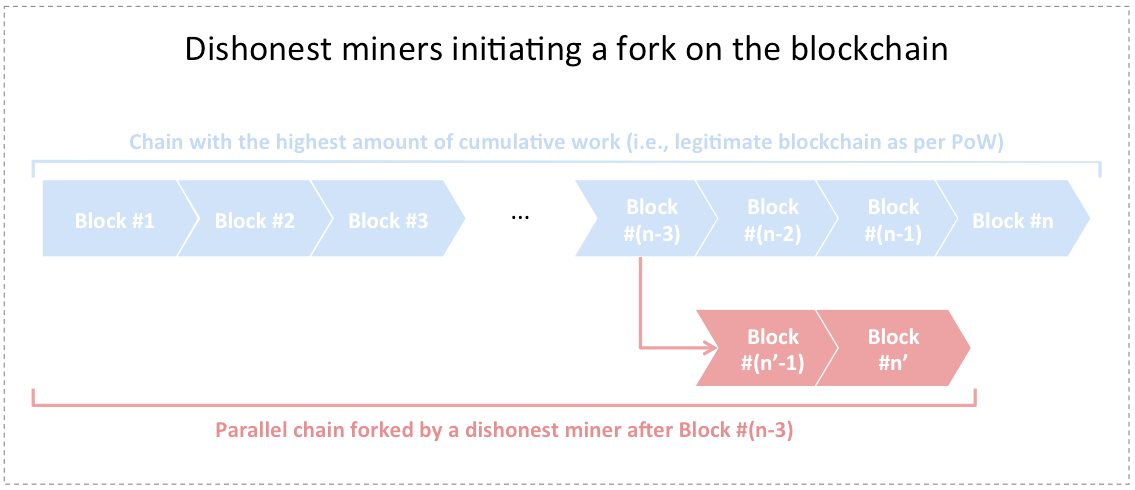
- Imperfection #2: There exists a subset of dishonest miners that decide to disregard the PoW consensus protocol. As a result, such miners can fork the blokchain and start mining on top of a parallel chain different than the one with the highest amount of cumulative work.
In the first case, miners are bound to momentarily experience diverging views of the blockchain. Even if all miners were honest, a network propagation delay would still cause natural forks to form on the blockchain. This is not desirable because one of the most important tenets of a well-functioning ledger consists in ensuring a unified view of the state of the system at any point in time.
We will show in section 2 that the probability of a natural fork occuring at some point in time on a system incurring an information propagation delay is equal to 1. However, we prove that the probability of sustaining a natural fork over a certain time interval is upper-bounded by a quantity that decays exponentially with the length of the interval. Consequently, any natural fork will collapse within finite time with high likelihood. A blockchain subject to the PoW consensus protocol is hence inclined to rapidly settle any natural fork that emerges.
In the second case, dishonest miners could stage an attack and maliciously attempt to redirect the blockchain to another chain of their liking and that suits their interest. The likelihood of success of such an attack (also known as a 51% attack) depends on the hashing power of the dishonest miner or pool of miners. We will discuss this case in section 3.
2. Probability of sustaining a natural fork when all miners are honest
We start by defining the following network parameters:
- Let
 denote the total number of miners on the network. We let
  denote the
  miner,
- Let
 denote ‘s hashing power, And let
  denote the network’s total hashing power.
 - Let
 denote the network’s block rate in units of blocks per second. Moreover, let
  denote ‘s specific block rate,
  . Hence
- Let
 denote the average time in seconds it takes to propagate a block from to
  and vice versa (assuming symmetry). We define the network’s average propagation delay to be
  We also define the network’s average propagation unit to be
- The probability that generates
 blocks (
 ) within an interval of
  seconds follows a Poisson distribution with mean equal to
  blocks. As a result,
  we have:
 generates blocks within
  seconds
 ![] = \frac{(\lambda_i t)^k}{k!}e^{-\lambda_i t}](https://delfr.com/wp-content/ql-cache/quicklatex.com-cf0e7dd5cda2be04bf0275596e0ce5a1_l3.png "Rendered by QuickLaTeX.com")
We also define the following four events:
 “At least one fork of the blockchain is formed at some point in time
 ![t_f \in (0, T]](https://delfr.com/wp-content/ql-cache/quicklatex.com-394cfe4d2de2f49e3f0e037a03e8ceb2_l3.png "Rendered by QuickLaTeX.com") “. The time origin
“. The time origin  can be chosen arbitrarily.
 “A fork is formed at block #
 of the blockchain. All miners shared a unified view of the blockchain right before #‘s addition.”
 “A fork that was created at time
  is sustained (i.e., does not collapse) for a minimum duration of
  seconds right after its formation.”
 “A double-spend transaction coexists with the legitimate transaction, seconds after the latter got added to a certain block” (We will discuss this event in more details later in this section).
Note that in what follows, we make the following two assumptions:
- The PoW consensus protocol consists in extending the chain of blocks that has the highest amount of accumulated work. Theoretically, this is not equivalent to the longest chain (i.e., the chain with the highest number of blocks). However, for all practical matters, we assume that they are equivalent going forward.
- The block propagation delay
 as defined earlier might be a large number since there might be nodes on the network that take a large amount of time on average to receive a given block. In general, block propagation statistics are described in terms of percentiles tracking how long it takes to propagate a block to a certain fraction of the network [2]. For all practical matters, we assume that corresponds to the average time taken to propagate a block to 99% of the network.
Our objective is four-fold:
- We first calculate the probability
![P[\mathcal{F}_{\infty}]](https://delfr.com/wp-content/ql-cache/quicklatex.com-ead7abf039bba2c62101007205fd54a5_l3.png "Rendered by QuickLaTeX.com") of a natural fork occuring at some point in time (assuming all miners are honest) and show it is equal to 1.
of a natural fork occuring at some point in time (assuming all miners are honest) and show it is equal to 1. - Second, we derive a non-trivial upper bound on
![P[\mathcal{D}^B],](https://delfr.com/wp-content/ql-cache/quicklatex.com-bc1b66b0ee660caaf585d70cdc6a12d5_l3.png "Rendered by QuickLaTeX.com") for any given block
for any given block 
- Third, we derive a non-trivial upper bound on
![P[\mathcal{S}_T],](https://delfr.com/wp-content/ql-cache/quicklatex.com-b8be7382a3f3ff444fdd00c7170e829f_l3.png "Rendered by QuickLaTeX.com") decaying exponentially in
decaying exponentially in 
- Finally, we derive a non-trivial upper bound on
![P[\mathcal{DS}_T],](https://delfr.com/wp-content/ql-cache/quicklatex.com-d383596e53ee32c1d85de6485f058941_l3.png "Rendered by QuickLaTeX.com") by making use of the results of the preceding two points.
by making use of the results of the preceding two points.
Objective #1: Natural forks on the blockchain happen with probability 1:
- Choose
 such that
  We can write:
![P[F_{\infty}] = lim_{n \rightarrow \infty} P[F_{nt_m}] = 1 - lim_{n \rightarrow \infty} P[\overline{F_{nt_m}}]](https://delfr.com/wp-content/ql-cache/quicklatex.com-9475d51ae4c8a1ffff44f54b15fd6aa4_l3.png "Rendered by QuickLaTeX.com")
where
 “No fork is formed on the blockchain at any time in the interval
 ![(0,nt_m]](https://delfr.com/wp-content/ql-cache/quicklatex.com-11dc85016b2488498939b4f98fc27499_l3.png "Rendered by QuickLaTeX.com") “
“  let
let  “No fork is formed on the blockchain at any time in the interval
 ![((k-1)t_m,\ kt_m]](https://delfr.com/wp-content/ql-cache/quicklatex.com-3d83e4b90369a7e078d713c76db2c5f3_l3.png "Rendered by QuickLaTeX.com") “. We can then write:
“. We can then write:

- Let
 “None of the
  miners generate any block in the interval “, and let
  “One and only one miner out of generates at least 1 block in the interval “. We claim that:
 for all
To see why, note that if both
 and
and  were not true, then there would exist at least two distinct miners that generate at least 1 block each in the interval
 ![((k-1)t_m,\ kt_m].](https://delfr.com/wp-content/ql-cache/quicklatex.com-43bfe49a55b77275bb462b3fa8692385_l3.png "Rendered by QuickLaTeX.com") But since
But since  it must be that at least two parallel blocks (one from each miner) coexist, hence forming a fork. Indeed, the choice of guarantees that none of the two blocks will have sufficient time to propagate to the other node. We conclude that
  is a necessary condition for
  to hold. Observing that and are disjoint, we get:
![P[E_{(k,t_m)}\ |\ \overline{F_{(k-1)t_m}}] \leq P[(E_0)_{(k,t_m)} \cup (E_1)_{(k,t_m)}] = P[(E_0)_{(k,t_m)}] + [(E_1)_{(k,t_m)}].](https://delfr.com/wp-content/ql-cache/quicklatex.com-e87d48c13220cbb32b2860b4fed52487_l3.png "Rendered by QuickLaTeX.com")
- We can calculate
![P[(E_0)_{(k,t_m)}] =\Pi_{i =1}^q e^{- \lambda_i t_m} = e^{-\lambda t_m}.](https://delfr.com/wp-content/ql-cache/quicklatex.com-09a5274f89b6245e1c91cdf569136688_l3.png "Rendered by QuickLaTeX.com") This quantity is independent of and so
This quantity is independent of and so ![P[(E_0)_{(k,t_m)}] \equiv P[(E_0)_{t_m}]](https://delfr.com/wp-content/ql-cache/quicklatex.com-220c644195a84b15a8e3dc367adc6e6b_l3.png "Rendered by QuickLaTeX.com")
- Similarly,
![P[(E_1)_{(k,t_m)}] = \Sigma_{i=1}^q [(1 - e^{-\lambda_i t_m}) \Pi_{j = 1, j \neq i}^q e^{-\lambda_j t_m}]](https://delfr.com/wp-content/ql-cache/quicklatex.com-3d6a0e23c78a9502ae5f8d0d70c6485f_l3.png "Rendered by QuickLaTeX.com")

This is also independent of
and so ![P[(E_1)_{(k,t_m)}] \equiv P[(E_1)_{t_m}]](https://delfr.com/wp-content/ql-cache/quicklatex.com-176dc5ca8e57c27741135e3e2619c3d9_l3.png "Rendered by QuickLaTeX.com")
- Putting it altogether, we get:
![P[\overline{F_{n \times t_m}}] = P[\cap_{k=1}^{n} E_{(k,t_m)}]\ =\ \Pi_{k=2}^{n}\ (P[E_{(k,t_m)}\ |\ \overline{F_{(k-1)t_m}}]) \times\ P[E_{(1,t_m)}]](https://delfr.com/wp-content/ql-cache/quicklatex.com-446d97c518c8db1e28497af64edba49b_l3.png "Rendered by QuickLaTeX.com")
![\leq \Pi_{k=2}^{n}\ (P[E_{(k,t_m)}\ |\ \overline{F_{(k-1)t_m}}])\ \leq\ \Pi_{k=2}^{n}\ (P[(E_0)_{t_m}] + P[(E_1)_{t_m}])](https://delfr.com/wp-content/ql-cache/quicklatex.com-e19f4b7e85470b39c0b4ca1bd8932cb6_l3.png "Rendered by QuickLaTeX.com")
![= (P[(E_0)_{t_m}] + P[(E_1)_{t_m}])^{n-1}](https://delfr.com/wp-content/ql-cache/quicklatex.com-82a998c6a000f9d54c50a846a5ea565c_l3.png "Rendered by QuickLaTeX.com")
 let
let  denote the event “
 and only miners out of generate at least 1 block each in an interval of seconds”. One can easily see that for a finite value of
 As a result, we have:
![P[(E_0)_{t_m}] + P[(E_1)_{t_m}] < \Sigma_{j=0}^q P[(E_j)_{t_m}] = 1](https://delfr.com/wp-content/ql-cache/quicklatex.com-8e52e96a8dbb61a9a31dc75accc7b7aa_l3.png "Rendered by QuickLaTeX.com")
- Consequently, we get:
![0 \leq P[\overline{F_{\infty}}] = lim_{n \rightarrow \infty} P[\overline{F_{nt_m}}]](https://delfr.com/wp-content/ql-cache/quicklatex.com-bf1b9f70cbe4f736a86d57ed8686add6_l3.png "Rendered by QuickLaTeX.com")
![\leq lim_{n \rightarrow \infty} (P[(E_0)_{t_m}] + P[(E_1)_{t_m}])^{n-1} = 0](https://delfr.com/wp-content/ql-cache/quicklatex.com-f74e0d682de5b91f237e77953cc0abf4_l3.png "Rendered by QuickLaTeX.com")
And since
![P[\overline{F_{\infty}}] = 0,](https://delfr.com/wp-content/ql-cache/quicklatex.com-f87b52ef676ee6df44add1a49f7f90f8_l3.png "Rendered by QuickLaTeX.com") we conclude that
we conclude that ![P[F_{\infty}] = 1](https://delfr.com/wp-content/ql-cache/quicklatex.com-41ef60abc4699be07356330792ad1769_l3.png "Rendered by QuickLaTeX.com")
Objective #2: A non-trivial upper bound on the probability of a natural fork occuring at an arbitrary block:
Suppose that all miners share a unified view of the blockchain. At time  one of the miners adds block # to the blockchain. Miners that still haven’t received block #
 (which for all practical matters could take up to
  could generate their own block and start a fork at #
 We are interested in computing the probability that such an event occurs, i.e.
 ![P[\mathcal{D}^B].](https://delfr.com/wp-content/ql-cache/quicklatex.com-ba1cdc538c68f7ae141d034c3791107f_l3.png "Rendered by QuickLaTeX.com") We define the following:
We define the following:
 “No fork ever gets formed at block #, knowing that all miners shared a unified view of the blockchain right before #‘s addition by some miner.”
 “None of the miners that still haven’t received block # by time
  , generate any block in
 ![(t_B + k \Delta t,\ t_B + (k+1) \Delta t].](https://delfr.com/wp-content/ql-cache/quicklatex.com-7738f58ef35a9f89e3d9e4898055ab85_l3.png "Rendered by QuickLaTeX.com") “
“- Let
 be the total number of miners out of a total of miners, that still haven’t seen block # by time
  Let these miners be indexed as
  and let
  denote the block rate of miner
By letting  we can write:

And so letting  we can write:
![P[\mathcal{U}^B] = lim_{\Delta t \rightarrow 0} \{{\Pi_{k=0}^{\infty}\ e^{-\Sigma_{j=1}^{q_{k, \Delta t}} (\lambda_{k_{j}} \Delta t)} \}}\ \geq\ lim_{\Delta t \rightarrow 0} \{{\Pi_{k=0}^{\infty}\ e^{- q_{k, \Delta t}(\lambda_{max} \Delta t)} \}}](https://delfr.com/wp-content/ql-cache/quicklatex.com-c40835088caf3b4aa5cb30f668de121c_l3.png "Rendered by QuickLaTeX.com")
![= lim_{\Delta t \rightarrow 0} \{{e^{- \Sigma_{k=0}^{\infty} [q_{k, \Delta t}(\lambda_{max} \Delta t)]} \}}\ =\ lim_{\Delta t \rightarrow 0} \{{e^{- \Sigma_{k=0}^{\infty} [(\frac{q_{k, \Delta t}}{q})(q \lambda_{max} \Delta t)]} \}}](https://delfr.com/wp-content/ql-cache/quicklatex.com-5bd7e9253a0062b581ce5d9fa6a70d70_l3.png "Rendered by QuickLaTeX.com")
Letting  be the ratio of miners that still haven’t received block # by time we get:
![P[\mathcal{U}^B] \geq e^{-q \lambda_{max} (\int_{0}^{\infty} g(t) dt)}](https://delfr.com/wp-content/ql-cache/quicklatex.com-7dba6ac6994eca2e84112e15222d1870_l3.png "Rendered by QuickLaTeX.com")
![P[\mathcal{D}^B] = 1 - P[\mathcal{U}^B] \leq 1 - e^{-q \lambda_{max} (\int_{0}^{\infty} g(t) dt)}](https://delfr.com/wp-content/ql-cache/quicklatex.com-a8b88bdf526d662acf4bba8cb52bafde_l3.png "Rendered by QuickLaTeX.com")
Note that if all miners share the same block rate  , then
  As a result, we would get
 ![P[\mathcal{D}^B] = 1 - e^{-\lambda (\int_{0}^{\infty} g(t) dt)}](https://delfr.com/wp-content/ql-cache/quicklatex.com-17b98c05d9f90fa1aa21c039afc5d99b_l3.png "Rendered by QuickLaTeX.com") (note the equality in this case). For small
(note the equality in this case). For small  this value can be approximated by
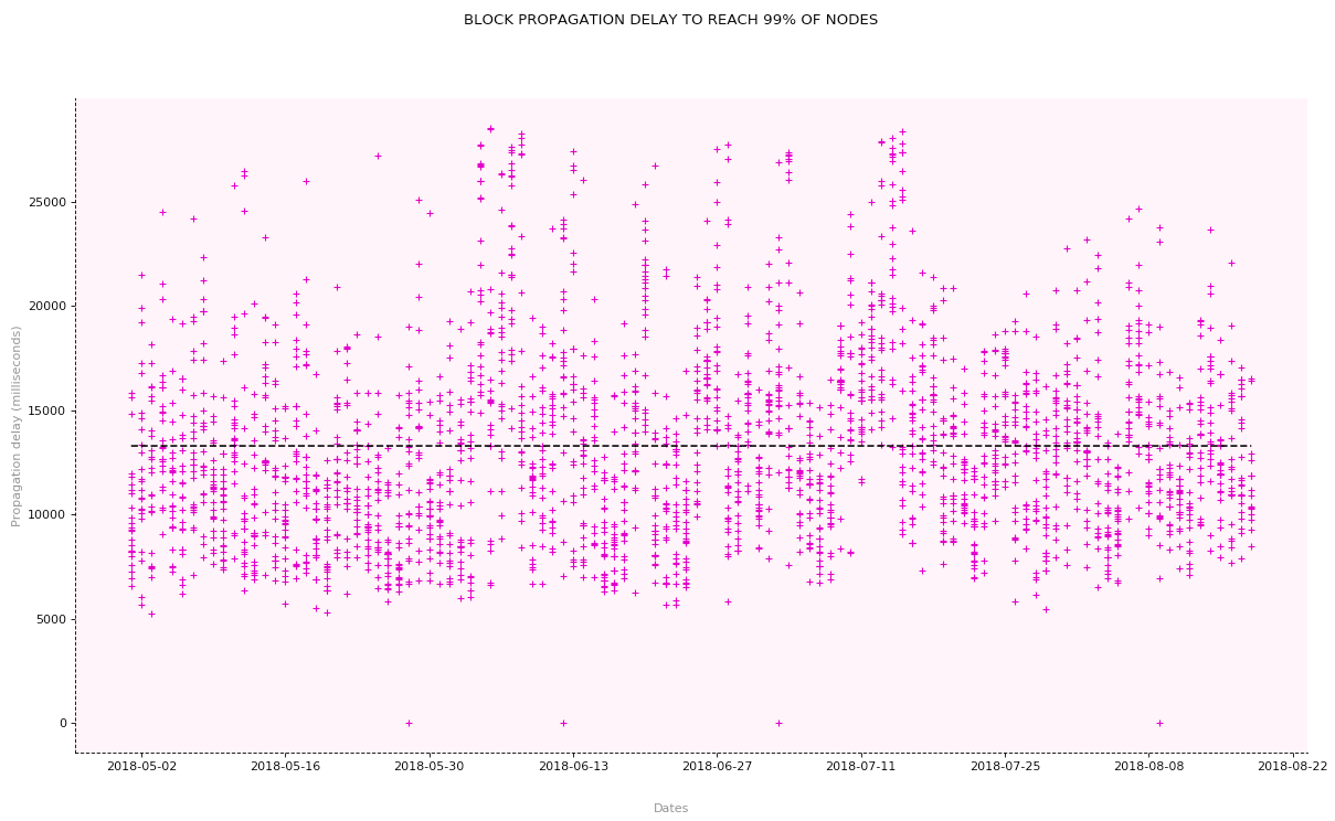
  as found in [1]. Below is a representation of a block propagation delay as observed on the
  of August 2018 [2]. In order to compute
  we make the assumption that the share of miners that still haven’t received the block by a certain time is the same as the corresponding share of generic nodes.
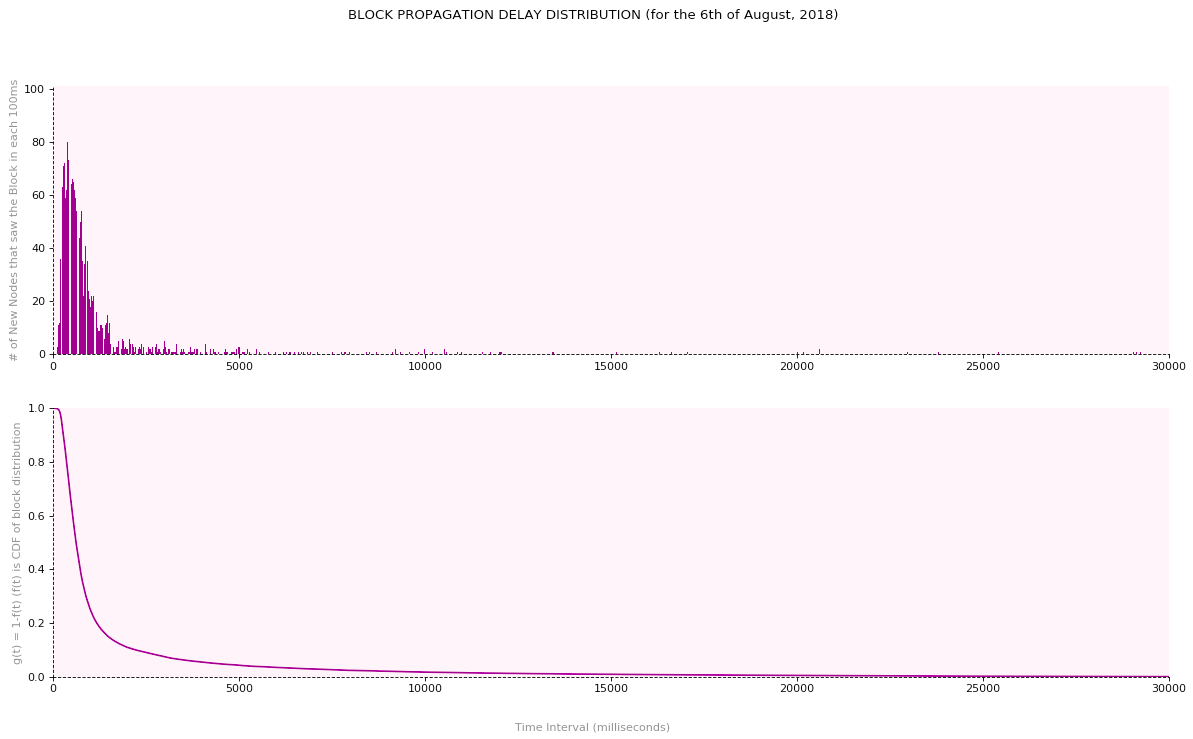
We find that  Using
Using  blocks/sec, we get
![P[\mathcal{D}^B] \leq 0.208%.](https://delfr.com/wp-content/ql-cache/quicklatex.com-941aeff997b84010c7402af01f46c44b_l3.png "Rendered by QuickLaTeX.com")
Objective #3: Natural forks collapse with high likelihood in a finite amount of time:
In what follows, we derive a non-trivial upper bound on ![P[S_T].](https://delfr.com/wp-content/ql-cache/quicklatex.com-084140b60d8c7400df159a57cd005c84_l3.png "Rendered by QuickLaTeX.com") To do so, we will first find a lower bound on the probability of occurrence of its complement
To do so, we will first find a lower bound on the probability of occurrence of its complement  “A fork that was created at time
  collapses at some point in time in the interval
 ![(t_f,\ t_{f + T}]](https://delfr.com/wp-content/ql-cache/quicklatex.com-2642215345344a86e4fe0d22cd28f018_l3.png "Rendered by QuickLaTeX.com") “. An adequate lower bound on
“. An adequate lower bound on ![P[\overline{S_T}]](https://delfr.com/wp-content/ql-cache/quicklatex.com-97a0caeafefab22e5acaeec5aaec4d96_l3.png "Rendered by QuickLaTeX.com") would be given by
would be given by ![P[E],](https://delfr.com/wp-content/ql-cache/quicklatex.com-d9f96d5c1cdeb58527fd0a1ee3f8e889_l3.png "Rendered by QuickLaTeX.com") where
where  is an event whose occurence is a sufficient condition for
  to hold true. Our objective becomes one of finding an appropriate and calculating a lower bound on
 ![P[E].](https://delfr.com/wp-content/ql-cache/quicklatex.com-ad18a259a43e730558d821029c9d1d2b_l3.png "Rendered by QuickLaTeX.com")
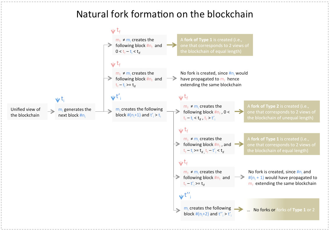
In the tree below, we depict the different scenarios that lead to a natural fork formation, starting with a shared view of the blockchain.  and
and  are time instances corresponding to block formations by miners and
  respectively. Recall that
  denotes the average block propagation time between and
  Scenarios that lead to a fork formation are one of two types: those that lead to parallel chains of equal length (i.e., Type 1) and those that lead to chains of different lengths (i.e., Type 2):
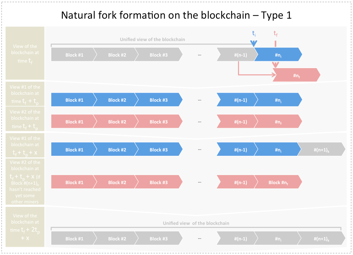
Forks of type 1: Before time  all miners share the same view of the blockchain. At
  (for some
  generates block #
 At
At  (for some
  generates the following block #
 such that
  If we wait for seconds and no miner generates any block in interval
 ![(t_f, t_f + t_p],](https://delfr.com/wp-content/ql-cache/quicklatex.com-73a596c570c8e5e648ae9513c111fa6e_l3.png "Rendered by QuickLaTeX.com") then at time
then at time  there will be more than one view of the blockchain, all of which have the same length. If for the following
  seconds (
 ), one and only one
  generates at least one block #
 , and then for the following seconds no miner generates any block, then by time
  all forks would collapse. This is depicted in the figure below:
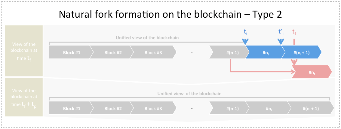
Forks of type 2: Before time  all miners share the same view of the blockchain. At (for some generates block # At
  mines the next block #
 At
At  (for some
  generates the following block #
 Two views of the blockchain will coexist at
  with one being a longer chain than the other. If we wait for seconds, and no miner generates any block in interval
 ![(t_f,\ t_f + t_p],](https://delfr.com/wp-content/ql-cache/quicklatex.com-59c4e79d21f064520f40adc4da8b559a_l3.png "Rendered by QuickLaTeX.com") then by all forks would collapse. This is depicted in the figure below:
then by all forks would collapse. This is depicted in the figure below:
One consequence is that given a fork that was formed at time , if we ensure that for the next seconds no miner generates any blocks, and that for the subsequent seconds one and only one miner generates at least 1 block, and finally for the subsequent seconds no miner generates any block, then the fork would collapse in the interval ![(t_f,\ t_f + x + 2t_p].](https://delfr.com/wp-content/ql-cache/quicklatex.com-fba7b0dae0958042640186bdca36d3d9_l3.png "Rendered by QuickLaTeX.com") This construction ensures a sufficient condition for a fork to collapse within a specific time interval. In what follows, we formalize our approach:
This construction ensures a sufficient condition for a fork to collapse within a specific time interval. In what follows, we formalize our approach:
- Let and let
 . We refer to as the interval design parameter expressed in units of seconds. We define the following events:
 “No miner out of generates any block in the time interval
 ![(t_f + k(x+2t_p),\ t_f + kx + (2k+1)t_p]](https://delfr.com/wp-content/ql-cache/quicklatex.com-1bf82d1e84f6a327b92d6b05ff55e9d9_l3.png "Rendered by QuickLaTeX.com") “
“ “One and only one miner out of generates at least 1 block in the time interval
 ![(t_f + kx + (2k+1)t_p,\ t_f + (k+1)x + (2k+1)t_p]](https://delfr.com/wp-content/ql-cache/quicklatex.com-59d9b26f0cfc57266122ef523cb84852_l3.png "Rendered by QuickLaTeX.com") “
“ “No miner out of generates any block in interval
 ![(t_f + (k+1)x + (2k+1)t_p,\ t_f + (k+1)(x + 2t_p)]](https://delfr.com/wp-content/ql-cache/quicklatex.com-aa2806db53cd0d49f3b0ef219745f71a_l3.png "Rendered by QuickLaTeX.com") “
“ “Any fork that could have existed at time
  collapses at some time in the interval
 ![(t_f + k(x+2t_p),\ t_f + (k+1)(x+2t_p)].](https://delfr.com/wp-content/ql-cache/quicklatex.com-8238b80f1f41302a4a74bd8c588504d1_l3.png "Rendered by QuickLaTeX.com") “
“ “At least one fork that existed at time is sustained throughout “
- The previous logic allows us to conclude that if
 and
and  are all satisifed, then
  will hold true
  and so will
 We conclude that the event
  is a sufficient condition for the occurence of
  and (
and ( We get:
![p[E_{(k,x)}],\ p[E_{(k,x)}\ |\ \overline{E_{(k-1,x)}},..., \overline{E_{(0,x)}}]\ \geq](https://delfr.com/wp-content/ql-cache/quicklatex.com-6f5267ea1cb0fd10cc6dc0692da59b6f_l3.png "Rendered by QuickLaTeX.com")
![p[(E_0)_{(k,x)} \cap (E_1)_{(k,x)} \cap (E_2)_{(k,x)}] \equiv](https://delfr.com/wp-content/ql-cache/quicklatex.com-30bbe37d586d4a9e8bab5e37bd1fafe6_l3.png "Rendered by QuickLaTeX.com")
 does not create any block in time interval
 ![(t_f + k(x+2t_p),\ t_f + kx + (2k+1)t_p])](https://delfr.com/wp-content/ql-cache/quicklatex.com-3ed23c7b202c7ee34ac0f06778b05065_l3.png "Rendered by QuickLaTeX.com")
 creates at least one block in time interval
 ![(t_f + kx + (2k+1)t_p,\ t_f + (k+1)x + (2k+1)t_p\ ]\cap_{j=1, j \neq i}^q(m_j](https://delfr.com/wp-content/ql-cache/quicklatex.com-6b4cfeaa257fca843d631f7892964052_l3.png "Rendered by QuickLaTeX.com") does not create any block in time interval
does not create any block in time interval ![(t_f + kx + (2k+1)t_p,\ t_f + (k+1)x + (2k+1)t_p])\}](https://delfr.com/wp-content/ql-cache/quicklatex.com-8ca1bd97cc20ea9818d40aabf1618342_l3.png "Rendered by QuickLaTeX.com")
 does not create any block in
 ![(t_f + (k+1)x + (2k+1)t_p,\ t_f + (k+1)(x + 2t_p)])\ ]](https://delfr.com/wp-content/ql-cache/quicklatex.com-061c952d2521f2173a5fffcc7308015b_l3.png "Rendered by QuickLaTeX.com")
Recognizing that all the events appearing under the union symbol above are disjoint, and that all the intersections are taken over independent events, we get:
![p[E_{(k,x)}],\ p[E_{(k,x)}\ |\ \overline{E_{(k-1,x)}},..., \overline{E_{(0,x)}}] \geq](https://delfr.com/wp-content/ql-cache/quicklatex.com-bb89eecfdad7d55b653514ba33440616_l3.png "Rendered by QuickLaTeX.com")
![[\Sigma_{i=1}^q (1-e^{-\lambda_i x}) e^{-(\lambda - \lambda_i)x}]e^{-2\lambda t_p}](https://delfr.com/wp-content/ql-cache/quicklatex.com-262ace5ef58fdf7b5fbef09820f04254_l3.png "Rendered by QuickLaTeX.com")
![=\ e^{-\lambda (x + 2t_p)}[\Sigma_{i=1}^q e^{\lambda_i x}\ -\ q]](https://delfr.com/wp-content/ql-cache/quicklatex.com-47ab3f1a0219d8315ea70fa3e3ea266d_l3.png "Rendered by QuickLaTeX.com")
- Now note that
 And since the exponential function is convex, we can invoke Jensen’s inequality to conclude that
  we have:

- As a result,

![P[(E)_{(k,x)}],\ P[E_{(k,x)}\ |\ \overline{E_{(k-1,x)}},..., \overline{E_{(0,x)}}] \geq\ q e^{-\lambda (x + 2t_p)}[e^{(\lambda x) / q} - 1]](https://delfr.com/wp-content/ql-cache/quicklatex.com-d43894652075be7449b3b3f61bfca50c_l3.png "Rendered by QuickLaTeX.com")
- And so
![P[\overline{E_{(k,x)}}] = 1 - P[E_{(k,x)}] \leq 1 - q e^{-\lambda (x + 2t_p)}[e^{(\lambda x) / q} - 1]](https://delfr.com/wp-content/ql-cache/quicklatex.com-a09a30e65f75565e72141bf161ca1c9d_l3.png "Rendered by QuickLaTeX.com")
![P[\overline{E_{(k,x)}}\ |\ \overline{E_{(k-1,x)}},..., \overline{E_{(0,x)}}] = 1 - P[E_{(k,x)}\ |\ \overline{E_{(k-1,x)}},..., \overline{E_{(0,x)}}] \leq](https://delfr.com/wp-content/ql-cache/quicklatex.com-ecc2c303f1b4b3d7cb6a4c6c9a25c957_l3.png "Rendered by QuickLaTeX.com")
![1 - q e^{-\lambda (x + 2t_p)}[e^{(\lambda x) / q} - 1]](https://delfr.com/wp-content/ql-cache/quicklatex.com-a6146cc61496d0e952659cac62627a4e_l3.png "Rendered by QuickLaTeX.com")
- Let
 In order to sustain a fork over a minimum duration of
  seconds after its formation at time we must sustain it over each
 ![(t_f + k(x + 2t_p),\ t_f + (k+1)(x + 2t_p)],\ \forall k \in \{{0,...,n-1\}}.](https://delfr.com/wp-content/ql-cache/quicklatex.com-c125980119565538e1bc9231c8ec2066_l3.png "Rendered by QuickLaTeX.com") This implies that:
This implies that:

As a result,
we can write:![P[\mathcal{S}_{n(x + 2t_p)}]\ \leq\ P[\cap_{k = 0}^{n-1} \overline{E_{(k,x)}}]\ =](https://delfr.com/wp-content/ql-cache/quicklatex.com-05715e2423d170316b8a521c679ac158_l3.png "Rendered by QuickLaTeX.com")
![\Pi_{k=1}^{n-1} P[\overline{E_{(k,x)}}\ |\ \overline{E_{(k-1,x)}},.., \overline{E_{(0,x)}}]\ \times\ P[\overline{E_{(0,x)}}] \leq](https://delfr.com/wp-content/ql-cache/quicklatex.com-ff16feaf405ae59f9f7f397282e04414_l3.png "Rendered by QuickLaTeX.com")
![(1 - q e^{-\lambda (x + 2t_p)}[e^{(\lambda x) / q} - 1])^n](https://delfr.com/wp-content/ql-cache/quicklatex.com-a8900bc33f71c475b7edaaecf154666d_l3.png "Rendered by QuickLaTeX.com")
And in particular,
![P[\mathcal{S}_{n(x + t_p)}]\ \leq\ min_{x > 0}(1 - q e^{-\lambda (x + 2t_p)}[e^{(\lambda x) / q} - 1])^n](https://delfr.com/wp-content/ql-cache/quicklatex.com-0599fb0602e922319b50ca74d17e28b2_l3.png "Rendered by QuickLaTeX.com")
- Finally, for a given time interval of seconds, we can write:
![P[\mathcal{S}_T]\ \leq\ min_{x > 0}(1 - q e^{-\lambda (x + 2t_p)}[e^{(\lambda x) / q} - 1])^{\lfloor{\frac{T}{x+2t_p}}\rfloor}](https://delfr.com/wp-content/ql-cache/quicklatex.com-7cdc169c6c58b7ab726b623b15ae9482_l3.png "Rendered by QuickLaTeX.com")
Where
 denotes the floor function.
The objective function of the previous optimization problem is not smooth due to the presence of the floor function. As a result, finding a closed form analytical solution might prove difficult. However, numerical methods could be employed to find the optimal upper bound. Observe that this upper bound decays exponentialy with and eventually converges to 0 when  . We use the value of
  that corresponds to the average block propagation delay to reach 99% of the network observed over a period of time extending from May
  2018 to August
  2018 [2].
Below, we include various graphs of this upper bound for different values of and for fixed  and
and 
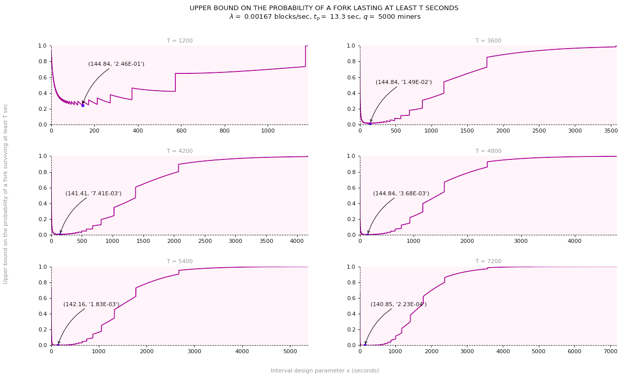
These graphs show that for the pre-defined values of  and
and  the probability that a natural fork survives
  minutes (which on average corresponds to the addition of 2 new blocks on the blockchain) is upper-bounded by 0.25 (or almost 1 in 4 cases). When
  minutes (i.e., the duration required to add an average of six new blocks on the blockchain), the upper bound goes down to 0.015 (or almost 1 in 67 cases). And when
  minutes, it goes down to 0.00022 (or almost 1 in 4500 cases).
In the graphs above, we assumed a fixed block rate of 1 block per 10 minutes. This is the value used by Bitcoin. For what it is worth, one could further optimize the upper bound over positive values of  For fixed
  and
and  the tightest upper bound becomes:
![min_{x, \lambda > 0}(1 - q e^{-\lambda (x + 2t_p)}[e^{(\lambda x) / q} - 1])^{\lfloor{\frac{T}{x+2t_p}}\rfloor}](https://delfr.com/wp-content/ql-cache/quicklatex.com-a038e1eb6edb39a7e83dea4bb67c73ec_l3.png "Rendered by QuickLaTeX.com")
In order to solve it, we first find the optimal value of  that solves the following optimization problem:
![min_{\lambda > 0} (1 - q e^{-\lambda (x + 2t_p)}[e^{(\lambda x) / q} - 1])^{\lfloor{\frac{T}{x + 2t_p}}\rfloor}](https://delfr.com/wp-content/ql-cache/quicklatex.com-4861ff5ae1b9a6fbe07e911fc9aabb4d_l3.png "Rendered by QuickLaTeX.com")
Note that since the exponent appearing in the objective function does not depend on and since the base is a positive quantity, we can solve the following equivalent optimization problem whose objective function is now smooth:
![min_{\lambda > 0} (1 - q e^{-\lambda (x + 2t_p)}[e^{(\lambda x) / q} - 1])](https://delfr.com/wp-content/ql-cache/quicklatex.com-e72507807c167119c1949ffed8e1e5d9_l3.png "Rendered by QuickLaTeX.com")
Note that when  or when
  the objective function tends to 1. The objective function turns out to be convex in and we can solve for
  by setting its first derivative with respect to equal to 0. Doing so, yields:

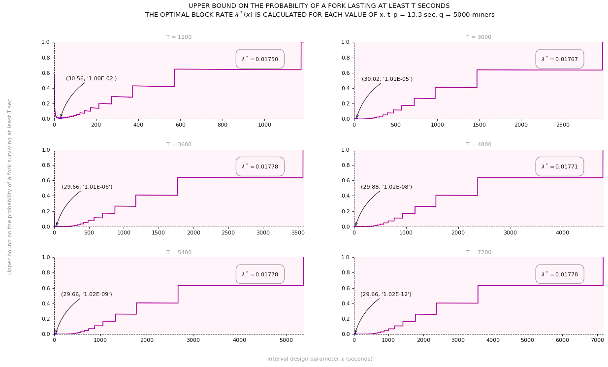
The tightest upper bound over all positive values of and then satisfies:
![min_{x > 0}(1 - q e^{-\lambda^* (x + 2t_p)}[e^{(\lambda^* x) / q} - 1])^{\lfloor{\frac{T}{x + 2t_p}}\rfloor}](https://delfr.com/wp-content/ql-cache/quicklatex.com-6f05769bca260e51b895ecc1720baab0_l3.png "Rendered by QuickLaTeX.com")
For each of the following graph, we let  and specify a particular value for For each value of
  we then calculate the corresponding
  as outlined above, and plot the graph of
![(1 - q e^{-\lambda^* (x + 2t_p)}[e^{(\lambda^* x) / q} - 1])^{\lfloor{\frac{T}{x + 2t_p}}\rfloor}:](https://delfr.com/wp-content/ql-cache/quicklatex.com-bdf5c2acc78ceea77d8be80b40755aa5_l3.png "Rendered by QuickLaTeX.com")
Objective #4: A non-trivial upper bound on the probability of a double-spend transaction coexisting with the legitimate transaction, seconds after the legitimate transaction is added to the blockchain:
The derivations above demonstrate that even if all miners were honest, forks are bound to happen, although they collapse with high likelihood after a finite time of their formation. The existence of natural forks could encourage dishonest customers to engage in double-spending behavior.
To see how, consider a scenario in which a customer spends some Satoshis to purchase a physical product. Let the transaction be denoted  Suppose that at
  the vendor sees his transaction
  included in block # for the first time on the blockchain. Suppose that the customer issues another transaction
  (before or after
  ) destined to himself and that uses the same UTXOs as There is a chance that both and be selected by two different miners and included in two separate coexisting blocks. We define the following double-spending event:
“ and coexist on the bockchain, seconds after ‘s addition to the blockchain in block  “
“
Note that if no fork is formed at or before block  then will not constitute a double-spending risk since would have propagated to all nodes. As a result, a necessary condition for a double-spending risk to exist consists of the union of the following events:
- “A fork is formed at block # of the blockchain and is added to this fork at some point in time. All miners shared a unified view of the blockchain right before #‘s addition”
 “A fork was formed at some block
  preceding and is added to this fork at some point in time. All miners shared a unified view of the blockchain right before #
 ‘s addition”
We would like to calculate a non-trivial upper bound on ![P[\mathcal{DS}_T].](https://delfr.com/wp-content/ql-cache/quicklatex.com-4705162a8789c1b94346be1f831cbf00_l3.png "Rendered by QuickLaTeX.com") We can write:
We can write:
![P[\mathcal{DS}_T] = P[\mathcal{DS}_T \cap \mathcal{D}^B] + P[\mathcal{DS}_T \cap \mathcal{D}^{B_p}]](https://delfr.com/wp-content/ql-cache/quicklatex.com-1bd42045fd5458394ffb7623affba3ad_l3.png "Rendered by QuickLaTeX.com")
-
![P[\mathcal{DS}_T \cap \mathcal{D}^B] = P[\mathcal{DS}_T\ |\ \mathcal{D}^B] \times P[\mathcal{D}^B]](https://delfr.com/wp-content/ql-cache/quicklatex.com-66a6f0caf010429c00839441fe1d6515_l3.png "Rendered by QuickLaTeX.com")
We saw earlier that
![P[\mathcal{D}^B] \leq 1 - e^{-q \lambda_{max} (\int_{0}^{\infty} g(t) dt)}.](https://delfr.com/wp-content/ql-cache/quicklatex.com-2ac83fc1efaf7ce03dc795cf9493d450_l3.png "Rendered by QuickLaTeX.com")
Moreover,
 And so,
![P[\mathcal{DS}_T\ |\ \mathcal{D}^B] \leq\ min_{x > 0}(1 - q e^{-\lambda (x + 2t_p)}[e^{(\lambda x) / q} - 1])^{\lfloor{\frac{T}{x+2t_p}}\rfloor}](https://delfr.com/wp-content/ql-cache/quicklatex.com-49224dd02b421936485f93c1e9008c47_l3.png "Rendered by QuickLaTeX.com")
Assuming that
 we get
![P[\mathcal{DS}_T\ |\ \mathcal{D}^B] \leq\ min_{x > 0}(1 - q e^{-\lambda (x + 2t_p)}[e^{(\lambda x) / q} - 1])^{\frac{T}{x+2t_p}-1}](https://delfr.com/wp-content/ql-cache/quicklatex.com-af10ddb555356a6fbfbb6809bb08e185_l3.png "Rendered by QuickLaTeX.com")
- Let be a non-negative integer and let
 be an arbitrary interval of time. Without loss of generality, assume block
  was added at
  Define
  “Block # preceding # was created in interval
 ![(-(k+1)\Delta t, -k \Delta t],](https://delfr.com/wp-content/ql-cache/quicklatex.com-b74eb03774f3b0ea0f583484ac7a7c9f_l3.png "Rendered by QuickLaTeX.com") a fork was formed at # and is added to this fork at some point in time. All miners shared a unified view of the blockchain right before #‘s addition”. We can write:
a fork was formed at # and is added to this fork at some point in time. All miners shared a unified view of the blockchain right before #‘s addition”. We can write:
![P[\mathcal{DS}_T \cap \mathcal{D}^{B_p}] = lim_{\Delta t \rightarrow 0}\ \Sigma_{k=0}^{\infty}\ P[\mathcal{DS}_T \cap \mathcal{D}^{B_{p,k}}]](https://delfr.com/wp-content/ql-cache/quicklatex.com-9eececabaaa73ef1e37e87cec84b8e0e_l3.png "Rendered by QuickLaTeX.com")
![= lim_{\Delta t \rightarrow 0}\ \Sigma_{k=0}^{\infty}\ P[\mathcal{D}^{B_{p,k}}] \times P[\mathcal{DS}_T\ |\ \mathcal{D}^{B_{p,k}}]](https://delfr.com/wp-content/ql-cache/quicklatex.com-1c554954be23e1f4ddcde1615ece168b_l3.png "Rendered by QuickLaTeX.com")
Note that
-
![P[\mathcal{D}^{B_{p,k}}]\ =\ P[\mathcal{D}^{B_{p,k}}\ \cap\ \mathcal{D}^{B_p}]\ =\ P[\mathcal{D}^{B_{p}}] \times P[\mathcal{D}^{B_{p,k}}\ |\ \mathcal{D}^{B_{p}}].](https://delfr.com/wp-content/ql-cache/quicklatex.com-1704431f8d76d28bb9dcd3abceb83c68_l3.png "Rendered by QuickLaTeX.com")
-
 At least one block added in the interval
 ![[-(k+1)\Delta t,\ -k \Delta t)].](https://delfr.com/wp-content/ql-cache/quicklatex.com-96159653f22d5c5d17944f50823da476_l3.png "Rendered by QuickLaTeX.com")
-

We then have:
![P[\mathcal{D}^{B_{p,k}}] \leq P[\mathcal{D}^{B_p}] \times P[](https://delfr.com/wp-content/ql-cache/quicklatex.com-7038e46353f0bc95ba737599174ae554_l3.png "Rendered by QuickLaTeX.com") at least one block is added in interval
at least one block is added in interval ![[-(k+1)\Delta t,\ -k \Delta t)]](https://delfr.com/wp-content/ql-cache/quicklatex.com-6fcfb5c343e74a6db07fa9c30993fe54_l3.png "Rendered by QuickLaTeX.com")
As a result,
![P[\mathcal{DS}_T \cap \mathcal{D}^{B_p}]\ \leq lim_{\Delta t \rightarrow 0}\ \{P[\mathcal{D}^{B_p}] \times](https://delfr.com/wp-content/ql-cache/quicklatex.com-524e63e6365bbf09035fc44d8f13dce7_l3.png "Rendered by QuickLaTeX.com")
![(1-e^{-\lambda \Delta t})\ \Sigma_{k=0}^{\infty}\ min_{x > 0}(1 - q e^{-\lambda (x + 2t_p)}[e^{(\lambda x) / q} - 1])^{\lfloor{\frac{T + k \Delta t}{x+2t_p}}\rfloor}\}](https://delfr.com/wp-content/ql-cache/quicklatex.com-468eec37198e4aab75ef1cb46acc67ad_l3.png "Rendered by QuickLaTeX.com")
Assuming
we get ![P[\mathcal{DS}_T \cap \mathcal{D}^{B_p}] \leq](https://delfr.com/wp-content/ql-cache/quicklatex.com-59ed56879a77d136b5ca6da5e60ab82b_l3.png "Rendered by QuickLaTeX.com")
![lim_{\Delta t \rightarrow 0}\ \{P[\mathcal{D}^{B_p}] \times](https://delfr.com/wp-content/ql-cache/quicklatex.com-53c23e1bd380fc7407ce71f923a82602_l3.png "Rendered by QuickLaTeX.com")
![(1-e^{-\lambda \Delta t})\ \Sigma_{k=0}^{\infty}\ min_{x > 0}(1 - q e^{-\lambda (x + 2t_p)}[e^{(\lambda x) / q} - 1])^{\frac{T + k \Delta t}{x+2t_p} - 1}\}](https://delfr.com/wp-content/ql-cache/quicklatex.com-c1546801676857414e1142f54d86ba0c_l3.png "Rendered by QuickLaTeX.com")
In the limit when
becomes infinitesimally small and tends to  the quantity
  tends to
  We can then write
![P[\mathcal{DS}_T \cap \mathcal{D}^{B_p}] \leq P[\mathcal{D}^{B_p}]\ min_{x > 0} \int_0^{\infty} \lambda (1 - q e^{-\lambda (x + 2t_p)}[e^{(\lambda x) / q} - 1])^{\frac{T + t}{x+2t_p} - 1} dt](https://delfr.com/wp-content/ql-cache/quicklatex.com-71daf6412b3de67b0698c24a89121292_l3.png "Rendered by QuickLaTeX.com")
![=P[\mathcal{D}^{B_p}]\ min_{x > 0}\ \frac{-\lambda (x + 2t_p)}{ln(1 - q e^{-\lambda (x + 2t_p)}[e^{(\lambda x) / q} - 1])} (1 - q e^{-\lambda (x + 2t_p)}[e^{(\lambda x) / q} - 1])^{\frac{T}{x+2t_p} - 1}](https://delfr.com/wp-content/ql-cache/quicklatex.com-fa0884b5726ae7d5ec072730f220de42_l3.png "Rendered by QuickLaTeX.com")
Similar to
![P[\mathcal{D}^{B}]](https://delfr.com/wp-content/ql-cache/quicklatex.com-945ee4e4d77b0314a477844fd6da42b4_l3.png "Rendered by QuickLaTeX.com") , we have
, we have![P[\mathcal{D}^{B_p}] \leq 1 - e^{-q \lambda_{max} (\int_{0}^{\infty} g(t) dt)}.](https://delfr.com/wp-content/ql-cache/quicklatex.com-0ce6b068523333ca22279802895b2419_l3.png "Rendered by QuickLaTeX.com")
-
We then conclude that ![P[\mathcal{DS}_T] \leq](https://delfr.com/wp-content/ql-cache/quicklatex.com-f1915f3b4e19ffacfbee3b16a6416f2b_l3.png "Rendered by QuickLaTeX.com")

![(1 - q e^{-\lambda (x + 2t_p)}[e^{(\lambda x) / q} - 1])^{\frac{T}{x+2t_p} - 1} (1 - \frac{\lambda (x + 2t_p)}{ln(1 - q e^{-\lambda (x + 2t_p)}[e^{(\lambda x) / q} - 1])})](https://delfr.com/wp-content/ql-cache/quicklatex.com-7cec8619de4eccb3f98ddb2c6840cd14_l3.png "Rendered by QuickLaTeX.com")
The graphs below depict the upper bound on the probability that a double spend transaction coexists with on the blockchain seconds after is added to block # for various values of and
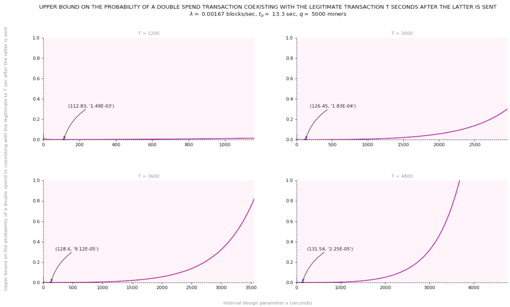
The above graphs show that if before handing over the goods, the vendor waits for an additional minutes after he sees added to block # on the blockchain (which at a block rate of
  would roughly correspond to two additional blocks on top of #), then for
  and all miners being honest and sharing the same hash rate, the probability of a double-spend attempt coexisting with at time is upper-bounded by 0.00149.
That means that there is at most a probability of 0.00149 that is still part of a parallel fork. By virtue of being sustained, it could still become part of the longest chain. If this happens, gets thrown back into the mempool and gets validated instead. On the other hand, waiting for an an additional  minutes (i.e., roughly 5 additional blocks on top of #), would bring down this probability to 0.000183.
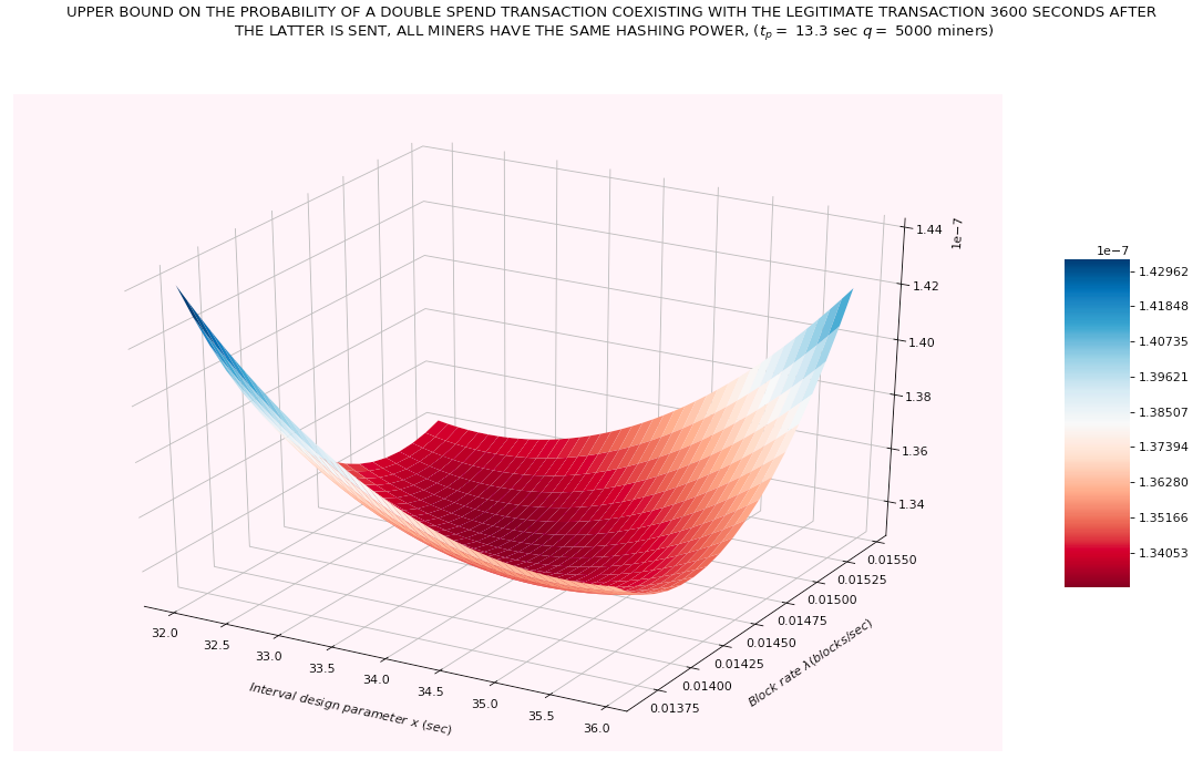
One could also optimize the upper bound not only over but also over Below is a plot showing the optimal value for the case minutes. In this case, the tightest upper bound is 1.33  which is achieved for
  blocks / sec and
  sec.
sec.
A small note on the value of  To the extent of our knowledge, the choice of used in Bitcoin is not the result of a pure mathematical optimization exercise. The larger the value of the higher the probability of a natural fork occuring. Natural forks are not desirable as they possibly pave the way to double-spending attempts. However, this is not the only metric that counts.
Another important consideration has to do with the storage capacity requirement and the rate of growth of such capacity that needs to be maintained at the level of each full node on the network. A higher means faster transaction processing but also faster growth of ever-increasing storage requirement. It is most likely that only a handful of nodes will be able to afford such storage, subsequently leading to a centralization scenario. This stands in sharp contrast with Bitcoin’s fundamental philosophy. As a result of this tradeoff, Satoshi’s choice of is probably a good compromise.
3. Probability that dishonest miner(s) succeed in creating a dominant fork: 51% attack
In this section we look at the second type of imperfections alluded to earlier. More specifically, we turn to the possibility that a subset of dishonest miner(s) decide to disregard the PoW consensus protocol and mine on top of a parallel chain different than the one with the highest amount of cumulative work.
This type of behavior has been introduced and analyzed in section 11 of Nakamoto’s seminal paper [3]. The analysis demonstrates that dishonnest miner(s) could possibly generate a parallel chain that overtakes the original honest chain. As a consequence, malicious miner(s) can potentially engage in double spending behavior.
Such a scenario is commonly referred to as a 51% attack, although malicious miner(s) do not necessarily need 51% of the total hashing power of the network to launch a double spending attack. A control of 51% or more of the total hashing power will however guarantee that the attack will be successful. On the other hand, control of less than 51% is not associated with a deterministic state of success, but rather a probabilistic one. The analysis in [3] quantifies the probability of success as a function of said control. In this section, we simply clarify the mathematical foundation of this analysis.
Building on the notation used in section 2, we further define the following quantities:
- Let
 be the subset of malicious miner(s) staging a 51% attack.
 - Let
 denote the fraction of the total hashing power controlled by the malicious miner(s). Note that in [3], this quantity is denoted by (in our notation, refers to the total number of miners).
 - Let
 denote the fraction of the total hashing power controlled by the honest miners.
 - Let
 correspond to the legitimate transaction against which
  will stage a 51% attack, and let be the block to which was initially added.
 - Let
 denote the interval of time extending from the moment was added to to the time the
  subsequent block following got added to the honest chain.
We also define the following two events:
 “The subset of malicious miner(s) with a fraction
  of the network’s total hashing power conduct a successful 51% attack on
  and has been previously validated by the addition of
  blocks on top of on the honest chain.”
 “The subset of malicious miner(s) with a fraction of the network’s total hashing power created and added blocks to the parallel chain in interval .”
We can write:
![P[\mathcal{A}^{51}_{r,z}] = \Sigma_{k = 0}^{\infty }\ P[\mathcal{A}^{51}_{r,z}\ \cap\ \mathcal{M}_{k,r,z}] = \Sigma_{k = 0}^{\infty }\ P[\mathcal{A}^{51}_{r,z}\ | \mathcal{M}_{k,r,z}] \times P[\mathcal{M}_{k,r,z}]](https://delfr.com/wp-content/ql-cache/quicklatex.com-eeb1d0c7869deec625435a135fc457c9_l3.png "Rendered by QuickLaTeX.com")
Calculating ![P[\mathcal{M}_{k,r,z}]](https://delfr.com/wp-content/ql-cache/quicklatex.com-614996b1f566005219433faf68eadbbd_l3.png "Rendered by QuickLaTeX.com") : Given a network block rate of blocks/sec, the rate associated with honest miners is
: Given a network block rate of blocks/sec, the rate associated with honest miners is  blocks/sec, and that associated with malicious miner(s) is
  blocks/sec. As a result,
  sec. In this interval, the subset of malicious miner(s) generate an average of
  blocks. As a result, we can model malicious miner(s) block generation over this inteval as a Poisson process with mean
  blocks. We get:
![P[\mathcal{M}_{k,r,z}] = \frac{(\frac{r}{p} z)^k\ e^{-\frac{r}{p} z}}{k!}](https://delfr.com/wp-content/ql-cache/quicklatex.com-78fc0adb8d5f0676160ac66f8fd8a491_l3.png "Rendered by QuickLaTeX.com")
Calculating ![P[\mathcal{A}^{51}_{r,z}\ | \mathcal{M}_{k,r,z}]](https://delfr.com/wp-content/ql-cache/quicklatex.com-022b1e209bce24e73db866165b957b38_l3.png "Rendered by QuickLaTeX.com") : Knowing that in interval the malicious miner(s) generated blocks on the parallel chain, we need to calculate the probability that the malicious miner(s) catch-up to the honest chain and generate a parallel chain that is at least as long (note that technically speaking, the parallel chain should be one block longer than the honest chain for the attack to be successful, but Nakamoto’s analysis considers the case of equal length instead). Clearly, if
: Knowing that in interval the malicious miner(s) generated blocks on the parallel chain, we need to calculate the probability that the malicious miner(s) catch-up to the honest chain and generate a parallel chain that is at least as long (note that technically speaking, the parallel chain should be one block longer than the honest chain for the attack to be successful, but Nakamoto’s analysis considers the case of equal length instead). Clearly, if  the probability is 1. When
  we can model the process as a binomial random walk whereby given that the malicious miner(s)’s parallel chain is
  blocks shorter than the honest chain:
- Every time the malicious miner(s) generate a new block, the gap gets reduced by 1.
- Every time the honest miners generate a new block, the gap gets increased by 1.
- Otherwise, the gap remains the same.
This problem turns out ot be a slight variant of the Gambler’s Ruin Problem that we introduce next.
- The Gambler’s Ruin Problem:
- The setting consists of a gambler who initially has units of currency (UOC for short).
- The gambler engages in a series of bets whereby every time she wins she gets UOC
 and every time she loses, she gives UOC
  .
. - Suppose that the gambler has a probability
 of winning each bet and a probability
  of losing. All bets are mutually independent.
 - The objective is for the gambler to reach a fortune of UOC
 before losing all her capital. As a result, the process will stop if either the gambler accumulates UOC
  or if she sees her capital reduced to 0.
In what follows, we calculate the probability that the gambler wins knowing that she started the game with UOC
 This is the probability that she reaches a fortune of UOC at some point in time knowing that she started off with UOC We denote it by
  A similar derivation can be found in [5] and [4]. Note that in this version of the game, the gambler cannot play if she does not have a positive amount of capital to start the betting process with. This stands in contrast to the aforementioned situation where malicious miner(s) start off with a block deficit. Later on, we will account for this variation.
We start by defining the following events:
{
 “The gambler wins”
{
 “The gambler wins the first bet in the series”
{
 “The gambler looses the first bet in the series”
And let
 be a random variable denoting the amount of capital held by the gambler at the beginning of the game.
We can write:
![P[\mathcal{W}\ |\ X=x] = P[\mathcal{W} \cap \mathcal{W}_1\ |\ X=x] + P[\mathcal{W} \cap \mathcal{L}_1\ |\ X=x]](https://delfr.com/wp-content/ql-cache/quicklatex.com-301ad464dc3101ede758ed48754ba2c3_l3.png "Rendered by QuickLaTeX.com")
![= P[\mathcal{W}\ |\ X=x,\ \mathcal{W}_1] \times P[\mathcal{W}_1\ |\ X=x] +](https://delfr.com/wp-content/ql-cache/quicklatex.com-0c1e92030737442425300c4c733fbd6b_l3.png "Rendered by QuickLaTeX.com")
![P[\mathcal{W}\ |\ X=x,\ \mathcal{L}_1] \times P[\mathcal{L}_1\ |\ X=x]](https://delfr.com/wp-content/ql-cache/quicklatex.com-3bf0e6b21e9a1d8cf13981aa2d327373_l3.png "Rendered by QuickLaTeX.com")
![= P[\mathcal{W}\ |\ X = x+1] \times P[\mathcal{W}_1\ |\ X=x]](https://delfr.com/wp-content/ql-cache/quicklatex.com-bb46f73f5b09b6490f81d3319c963bdf_l3.png "Rendered by QuickLaTeX.com")
![+ P[\mathcal{W}\ |\ X=x-1] \times P[\mathcal{L}_1\ |\ X=x]](https://delfr.com/wp-content/ql-cache/quicklatex.com-f0cb65a0bcac766e56dc70f09289cd2d_l3.png "Rendered by QuickLaTeX.com")
In other terms, we have:


 since
since 
Recognizing a telescoping series structure, we write:
![w_{(f, x+1)} - w_{(f, 1)} = \Sigma_{j=1}^x (w_{(f, j+1)} - w_{(f, j)}) = [\Sigma_{j=1}^x (\frac{l}{w})^j].\ w_{(f, 1)}](https://delfr.com/wp-content/ql-cache/quicklatex.com-214b413f3d98ddab86744a57b7b7eb55_l3.png "Rendered by QuickLaTeX.com")
And so,
![w_{(f, x)} = [\Sigma_{j=0}^{x-1} (\frac{l}{w})^j].\ w_{(f, 1)} =](https://delfr.com/wp-content/ql-cache/quicklatex.com-58ce33c41f4b4610111ea90a1113bd54_l3.png "Rendered by QuickLaTeX.com")
![[\frac{1 - (\frac{l}{w})^{x}}{1 - \frac{l}{w}}].\ w_{(f, 1)},](https://delfr.com/wp-content/ql-cache/quicklatex.com-d20677ccea1401ebd863f65ea591a212_l3.png "Rendered by QuickLaTeX.com") if
if 
 if
if 
Noting that
 and applying the above when
  we get
![1 = [\frac{1 - (\frac{l}{w})^{f}}{1 - \frac{l}{w}}].\ w_{(f, 1)}\ ,](https://delfr.com/wp-content/ql-cache/quicklatex.com-a9c380e8d085b2bc8c59680cdd5e348f_l3.png "Rendered by QuickLaTeX.com") if
if  if
if Which then allows us to conclude that

![[\frac{1 - \frac{l}{w}}{1 - (\frac{l}{w})^{f}}],\](https://delfr.com/wp-content/ql-cache/quicklatex.com-a18250b5b1bf6e405a2e35263f12f82b_l3.png "Rendered by QuickLaTeX.com") if
if  if
if Putting it altogether, we get

![\frac{1 - (\frac{l}{w})^{x}}{1 - (\frac{l}{w})^{f}}],](https://delfr.com/wp-content/ql-cache/quicklatex.com-4b06f29e7da228fc4094a46ad2ac3a88_l3.png "Rendered by QuickLaTeX.com") if
if  if
if - The setting consists of a gambler who initially has
- Adapting the Gambler’s Ruin Problem to the case of a 51% attack: In the context of a 51% attack, and for is the probability that the subset of malicious miner(s) catch up to the honest chain when the malicious miner(s)’ parallel chain is blocks behind. In other terms, the malicious miner(s) have a deficit of blocks at the beginning of the process and we are interested in calculating the probability that they catch-up at some point in time.
Note that under this setting, the block deficit may widen without having any lower-bound constraint.In the setting of the Gambler’s Ruin Problem, the gambler cannot play when she is in a deficit and will have to stop as soon as her betting capital reaches 0. As such, the problem must be modified to account for a scenario where the gambler could borrow unlimited credit if need be, to continue playing the game.
An equivalent formulation consists of a gambler having an infinite amount of capital to start with. Formally, we assume the same setting as the original problem. The gambler however, has a deficit of UOC
 . She then borrows UOC
  and starts the game with the objective of reaching UOC where
  . If she wins, she returns UOC to her creditor and keeps UOC so as to break-even. In case she loses, she does not return anything to her creditor.
Clearly, the above setting is unrealistic due to the dearth of extremely benevolent creditors. However, when we are dealing with a deficit of a block nature rather than a monetary one, this setting becomes acceptable. We then let
 and compute the corresponding probability of success. In our block deficit case,
  blocks.
We get
![lim_{x \rightarrow \infty}\ [w_{(x+(z-k),\ x)}] =](https://delfr.com/wp-content/ql-cache/quicklatex.com-3f3845c2dc4ef82ded00202ffd0ec597_l3.png "Rendered by QuickLaTeX.com")
![lim_{x \rightarrow \infty}\ [\frac{1 - (\frac{l}{w})^{x}}{1 - (\frac{l}{w})^{x+(z-k)}}],](https://delfr.com/wp-content/ql-cache/quicklatex.com-c1825720dd49187ac7e87301f58d74b0_l3.png "Rendered by QuickLaTeX.com") if
if ![lim_{x \rightarrow \infty}\ [\frac{x}{x+(z-k)}],](https://delfr.com/wp-content/ql-cache/quicklatex.com-f55c7599bbaecab65f6096071ddd7c58_l3.png "Rendered by QuickLaTeX.com") if
if Next, note that if
 then
then  And so
![lim_{x \rightarrow \infty}\ [\frac{1 - (\frac{l}{w})^{x}}{1 - (\frac{l}{w})^{x+(z-k)}}] = lim_{x \rightarrow \infty}\ [\frac{(\frac{l}{w})^{-x} - 1}{(\frac{l}{w})^{-x} - (\frac{l}{w})^{(z-k)}}] = (\frac{w}{l})^{(z-k)}](https://delfr.com/wp-content/ql-cache/quicklatex.com-2745b3cdc40830e8a2f07d40f1123148_l3.png "Rendered by QuickLaTeX.com")
And if
 then
then  And so
![lim_{x \rightarrow \infty}\ [\frac{1 - (\frac{l}{w})^{x}}{1 - (\frac{l}{w})^{x+(z-k)}}] = 1](https://delfr.com/wp-content/ql-cache/quicklatex.com-437cd0c80696dd95248a127fe08e0e7f_l3.png "Rendered by QuickLaTeX.com")
Finally, if
 then
then ![lim_{x \rightarrow \infty}\ [\frac{x}{x+(z-k)}] = 1.](https://delfr.com/wp-content/ql-cache/quicklatex.com-ec5a88f052fdf27fdf2c4d066ce163e3_l3.png "Rendered by QuickLaTeX.com")
As a result,
![lim_{x \rightarrow \infty}\ [w_{(x+(z-k),\ x)}] = (\frac{w}{l})^{(z-k)}](https://delfr.com/wp-content/ql-cache/quicklatex.com-bb114eb9b1e4b206fe0ca4cad01d236c_l3.png "Rendered by QuickLaTeX.com") if
if  and if
If malicious miner(s) are not incurring a block deficit, i.e.,
then![P[\mathcal{A}^{51}_{r,z}\ | \mathcal{M}_{k,r,z}] = 1](https://delfr.com/wp-content/ql-cache/quicklatex.com-189ffb701378b1dd8008d3336303c702_l3.png "Rendered by QuickLaTeX.com")
Otherwise, if
then noting that the probability of malicious miner(s) finding the next block is equal to and the one corresponding to the honest miners is equal to  we get:
![P[\mathcal{A}^{51}_{r,z}\ | \mathcal{M}_{k,r,z}] = (\frac{r}{p})^{(z-k)}](https://delfr.com/wp-content/ql-cache/quicklatex.com-131dfd32db25035dd72fa4101f768ad7_l3.png "Rendered by QuickLaTeX.com") if
if  and if
The calculations above allow us to conclude that:
![P[\mathcal{A}^{51}_{r,z}] = \Sigma_{k = 0}^{z-1}\ [\frac{(\frac{r}{p} z)^k\ e^{-\frac{r}{p} z}}{k!} (\frac{r}{p})^{(z-k)}]\ +\ \Sigma_{k = z}^{\infty }\ [\frac{(\frac{r}{p} z)^k\ e^{-\frac{r}{p} z}}{k!}]](https://delfr.com/wp-content/ql-cache/quicklatex.com-75a35c92085ca8d7592d991a3d9eada7_l3.png "Rendered by QuickLaTeX.com")
![= \Sigma_{k = 0}^{z-1}\ [\frac{(\frac{r}{p} z)^k\ e^{-\frac{r}{p} z}}{k!} (\frac{r}{p})^{(z-k)}]\ +\ 1 - \Sigma_{k = 0}^{z-1}\ [\frac{(\frac{r}{p} z)^k\ e^{-\frac{r}{p} z}}{k!}]](https://delfr.com/wp-content/ql-cache/quicklatex.com-71a64ca251c11c0104271e48de08a0ed_l3.png "Rendered by QuickLaTeX.com")
![= 1 - \Sigma_{k = 0}^{z-1}\ [\frac{(\frac{r}{p} z)^k\ e^{-\frac{r}{p} z}}{k!}][1 - (\frac{r}{p})^{(z-k)}],](https://delfr.com/wp-content/ql-cache/quicklatex.com-a362ee2c862d855822207189756111fd_l3.png "Rendered by QuickLaTeX.com") if
if 
and ![P[\mathcal{A}^{51}_{r,z}] = \Sigma_{k = 0}^{\infty }\ [\frac{(\frac{r}{p} z)^k\ e^{-\frac{r}{p} z}}{k!}] = 1,](https://delfr.com/wp-content/ql-cache/quicklatex.com-6bed00d89c2dec473eb30bbe20593cf8_l3.png "Rendered by QuickLaTeX.com") if
if
In the graphs below we plot the probability of a successful 51% attack as a function of the fraction of the total hashing power controlled by the subset of malicious miner(s). We do so for different values of the block validation height 
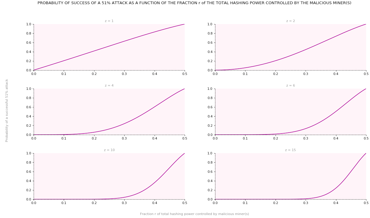
For example, assuming that malicious miner(s) controlled 15% of the total hashing power of the network (i.e.,  ), then a block validation height of 6 blocks (i.e.,
  ) is associated with a probability of a successful attack of 0.268%.
4. References
[1] Christian Decker and Roger Wattenhofer. Information propagation in the bitcoin network, 2013.
[2] DSN. Block propagation delay history.
[3] Satoshi Nakamoto. Bitcoin: A peer-to-peer electronic cash system. White Paper, 2008.
[4] A. Pinar Ozisik and Brian Neil Levine. An explanation of nakamoto’s analysis of double-spend attacks, online, 2017.
[5] Karl Sigman. Gambler’s ruin problem, online, 2016.
Tags: 51%, attack, blockchain, double spend, fork, miner
No comments
Comments feed for this article
Trackback link: https://delfr.com/blockchain-fork-analysis/trackback/