Consensus in distributed systems

November 16, 2020 in Bitcoin | No comments

Download pdf here: Consensus in distributed systems

1. Introduction

In the physical realm, paper fiat currencies are almost impossible to duplicate. As a result, a spent US Dollar bill cannot be concurrently used by the same payor in a different transaction. In digital space, one could also rule out double spending occurrences by setting up a central arbiter. In this case, the central authority (e.g., a bank) would decide on the fate of a transaction and enforce consensus. However, such central arbiters do not exist in decentralized structures. Up until Bitcoin, all decentralized attempts suffered from the possibility of duplicating digital units and spending them more than once.

Any decentralized solution to the double spending problem requires the relevant participants to reach consensus and agree on the ordering of transactions. This will ensure the recording of when digital unit(s) of money were spent and invalidate any attempt by their previous owner to reuse them. Bitcoin’s innovation lies in its ability to offer such a solution even when a minority of participants may act maliciously. The elements of the Bitcoin Consensus (also known as the Nakamoto Consensus) span transactions, blocks and the blockchain. We will discuss them in a subsequent post. In this chapter, we introduce the problem of reaching consensus in distributed systems, of which the Bitcoin network is an instance.

In section 2, we provide a brief introduction to these systems and highlight the intimate bond between a consensus problem and the underlying system parameters. The set of relevant parameters typically includes the network topology, the nodes configuration, the reliability of the communication channel, the synchronicity model, the types of messages exchanged, the failure regime of nodes, and whether consensus is achieved in a deterministic or a randomized way.

In section 3, we discuss the classical Byzantine Generals Problem (BGP) introduced by Lamport et al. [5], [6]. The classical BGP result is easy to state but its proof is not necessarily straightforward. Given its importance and historical value, we revisit the proof in the hope of making it easier to follow. The Byzantine Generals Problem became an allegorical representation of that of reaching consensus in distributed systems. It is commonly stated that “Bitcoin solves the BGP”. However, Bitcoin’s consensus problem is defined on a system whose parameters differ from those of the classical BGP. We will revisit this in a subsequent post.

In section 4, we look at a different class of system models which includes fully asynchronous distributed systems over which consensus must be achieved deterministically. We state and prove the seminal result that such a consensus is impossible to achieve in the presence of even a single faulty node. This is known as the FLP impossibility result in reference to its authors Michael J. Fischer, Nancy Lynch, and Mike Paterson.

2. Distributed systems

We define a distributed system to be a set of nodes spread-out across space. Each node runs a distinct process and can communicate with other nodes. For all practical matters, one can think of a node as a separate computer and the act of running-a-process as that of executing a specific task or computation. Moreover, a client that uses the distributed system does not perceive its nodes as separate entities but rather as part of a unit. In this unit, processes are executed in order to achieve a common purpose.

It is conceivable for a given node to run a process while at the same time be in control of its rules of execution (e.g., mandate when to run a process). In general however, one cannot necessarily assume that execution and governance (i.e., the particular model of control or ownership) are carried out by the same entity. A centralized governance is one where the ruling over the system is concentrated (e.g., in an individual, an organization, a state). On the other hand, the ruling in a decentralized system is spread over multiple entities.

An important implication is that a distributed system can be centralized. For example, Facebook runs a centralized model where decision-making power is concentrated within the organization. It remains nevertheless a distributed system where different servers and computers implement different processes. Bitcoin on the other hand, is an example of a distributed system that is also decentralized for anyone can join or leave the network and run an independent node.

In what follows, we describe some of the merits of distributed systems. We also showcase the importance of reaching agreement in such structures and highlight some of the challenges of doing so in the presence of faults. We finally introduce the notion of consensus and the parameters that characterize its associated system model.

The merits of a distributed system – In order to better appreciate the value of a distributed system, we mention three of its potential advantages over its non-distributed counterpart:

Better scaling: In a scenario where a particular node receives excessive traffic, there may be a threshold beyond which the node’s performance becomes noticeably impacted. One could upgrade the processing power of the node but the merits of this vertical scaling are bound to reach a limit. A more suitable alternative would be to distribute the workload by adding more nodes to the system.
Higher resilience: In a single-node system, any failure could be severely damaging. In order to mitigate the risk of a single-point failure and increase the level of tolerance for faulty behavior, one can create more redundancy by adding more nodes.
Lower latency: If the system’s clients were spread across the globe, information would have to travel for longer distances resulting in longer latencies. This can be improved by geographically distributing a richer set of nodes.

The need for agreement in a distributed system – In a distributed system where different nodes run their own processes, communicate with each other, and alter their perceptions of the state of the system accordingly, these nodes may end up having different concurrent views of the system. The need to agree on a common view is imperative in certain cases as highlighted by the following examples:

1) The distributed Transaction-Commit problem: A transaction gets divided into processes run by different nodes. The objective is to decide whether or not to commit the transaction to a given database. The important consideration is that if any node rejects it, then all nodes must do so too. Otherwise, the system’s view will be inconsistent as some nodes agree to include it while others don’t. A commitment of the transaction must occur if and only if all relevant nodes agree to do so.

2) State Machine Replication (SMR) systems: A state machine reflects the state of a system at a given point in time. It takes a set of inputs or commands, performs a set of operations (collectively defining a transition function), and then computes an output used to update the state of the system. An SMR distributed system consists of various nodes that are all supposed to run the same transition function. In order to ensure a consistent view of the system’s state, there needs to be agreement on the inputs to the transition function i.e., the current state of the system as well as inputs used to alter it.

A client may send a number of sequential requests to an SMR system. The ordering of these requests is paramount and any two nodes executing them out of order will have two conflicting views of the state of the system. This is known as the log replication problem (it is a reference to the idea that the sequence of commands is stored in a log). Assuming that all nodes operate the same deterministic transition function, an agreement in this context corresponds to an alignment among all nodes on the sequencing of the commands.

One important example of an SMR is the Bitcoin ledger. The state of the system at a given time corresponds to the set of Unspent Transaction Outputs (UTXO) (the reader can refer to Bitcoin Transactions (pre-segwit) for an introduction to UTXOs). Simply stated, this set corresponds to all public keys holding unspent satoshis. Inputs that alter the state of the ledger consist of valid Bitcoin transactions. Transactions however must be executed in a well-defined sequence agreed upon by all nodes. Otherwise, a Bitcoin transaction considered as valid by one node could be invalidated by another. We will discuss the building blocks and details of the Bitcoin consensus protocol in a later post.

3) Clock synchronization: In order for a system’s nodes to execute certain processes in a well-defined order, they need to share a common view of time. The challenge is that the internal clocks of nodes differ in the way they count the passage of time. The difference is due to clock drift, usually caused by relativistic effects. Clock synchronization is the problem of coordinating the clocks of various nodes at regular time intervals to ensure ordered execution of events. This problem can be equivalently stated as one of reaching agreement on a common value of time between various nodes.

The challenge of reaching agreement in the presence of faults – In light of the above examples, it becomes clear that some distributed systems must ensure that their nodes reach agreement. In a perfect world where nodes relay information truthfully, agreement could be easily achieved. For example, each node could be requested to relay its information to peers and then have all nodes apply a common function. Nodes however, may not be truthful all the time. In general, one assumes that a certain maximal number of them can be faulty. The behavior of faulty nodes is specified by a pre-defined failure model which may consist of:

Crash failure: In this model, a node can either be fully operational or out of order. In particular, a node may fail in the middle of an execution. As a result, it could have sent information to only a small subset of its peers before crashing.
Omission failure: Information sent by a node may not be received by a peer. This can be due to various factors including transmission problems or buffer overflow.
Byzantine failure: Byzantine faults are the weakest form of failures in the sense that faulty nodes can behave arbitrarily without abiding by specific constraints. In a byzantine regime, a faulty node can act maliciously vis-a-vis one of its peers at a certain time instance and honestly at another. In this context, malicious behavior is to be understood in its general form including e.g., communicating wrong information to peers or abstaining from sending or relaying any information. These faults are particularly important in a decentralized setting.

Consensus in distributed systems – The real challenge with distributed systems is to reach agreement in the presence of faulty behavior. More formally, the act of reaching agreement is encapsulated in the notion of achieving consensus. An algorithm is said to achieve consensus in a distributed system if it guarantees that the following three criteria are met:

Agreement: All non-faulty nodes (also known as correct nodes) must agree on the value (or array of values) that they compute. In other words they must all share the same value(s) after the algorithm is executed.
Validity: In the absence of any constraint, non-faulty nodes could agree on trivial values irrespective of the nature of the problem. In order for them to be meaningful, agreed-upon values must satisfy more stringent constraints. The validity criterion ensures that non-faulty nodes decide on “acceptable” value(s) for some notion of “acceptable”. Different validity requirements lead to different types of consensus.
Termination: All non-faulty nodes must eventually decide on a value (or array of values).

The above consensus criteria are usually expressed in terms of safety and liveness properties. Informally, safety is a property that must be continuously observed by the system in order to ensure that no “bad” outcome occurs. Liveness on the other hand, guarantees that a “good” outcome will eventually take place. Liveness properties do not need to be continuously observed but must eventually be met:

The Agreement criterion ensures that non-faulty nodes never diverge in their decision making. It is thus considered a safety property.
The Validity criterion guarantees that non-faulty nodes never choose an inadequate value. As a result, it is also considered a safety property.
The Termination criterion on the other hand, guarantees that eventually every non-faulty node will decide on a value. It is hence a liveness property.

The aforementioned Termination criterion requires that for each and every iteration of the consensus algorithm, non-faulty nodes decide on a value (or array of values). This definition characterizes a class of consensus algorithms known as deterministic. Termination could also be defined stochastically, leading to the class of randomized consensus algorithms. In this case, it becomes:

Termination: All non-faulty nodes must eventually decide on a value (or array of values) with probability 1.

In other words, some executions of the algorithm may fail to terminate as long as the probability of it happening approaches 0 when the number of executions tends to infinity.

System model specification – The characterization of a distributed system requires specifying a number of system parameters. They include:

Nodes configuration: A system may consist of a pre-defined set of static nodes that never changes over the course of execution. For instance, nodes could be geographically spread servers deployed by an organization to service its global client base. Configurations could also be dynamic (e.g., Bitcoin) with different nodes joining or leaving at various points in time.
Network topology: Nodes may be connected in various ways. For instance, a node can be linked to a select set of peers or to every other node as part of a complete graph topology.
Communication channel reliability: In addition to specifying the failure regime of nodes, a full description of a distributed system requires defining the reliability of its underlying communication channel. For all practical purposes, we will assume that the infrastructure is reliable and limit faulty behavior to nodes.
Communication delay: A system can be classified as synchronous, partially synchronous or fully asynchronous. In a synchronous network, messages sent are guaranteed to be delivered to peers within a fixed delay of $\Delta$ seconds known a priori. This presupposes that nodes have a common reference time against which $\Delta$ is measured and is typically achieved through clock synchronization at regular intervals called rounds. One advantage of synchronous systems is that nodes can recognize if a message has not been sent by waiting $\Delta$ seconds from the beginning of a specific round.
A more realistic model is that of an asynchronous network where no guarantees are imposed on message delivery delay except for the assurance that messages sent will eventually be delivered. Contrary to the synchronous case, asynchronous networks do not rely on a notion of a common reference time. An important result in distributed systems theory is the impossibility of achieving deterministic consensus in a fault-tolerant asynchronous setting. This is the FTP impossibility result [4] that we will discuss in section 3. The result ceases to hold if the deterministic constraint is replaced by its randomized counterpart [1], underscoring as such the importance of specifying the system parameters prior to solving for consensus.
A model that lies midway between these two extremes, is the partially synchronous one [2]. Partial synchrony comes in different flavors. One version assumes the existence of a not known a priori upper-bound $\Delta$ on the delay to deliver a message from one node to a peer. Another version assumes that the bound is known a priori but only guaranteed to apply starting at an unknown time instance.
Message authentication: Two types of messages could affect the process of reaching consensus in distributed systems. Unauthenticated or oral messages can be tampered with. A malicious node could modify the content of a message it received before it relays the altered version to a peer. It could also create a message and claim that it received it from a peer. Authenticated or signed messages on the other hand, are tamper-proof and forgery attempts will be detected with overwhelming probability. As a result, solving for consensus with signed messages is generally easier because the arsenal of malicious weapons does not include forgery.

In summary, consensus in distributed systems depends on a number of parameters. In order to specify a consensus problem, one needs to define:

The system parameters including the nodes configuration and topology, reliability of the channel, synchronicity model, and types of messages.
The faulty nodes failure regime (e.g., byzantine).
The nature of the Termination criterion (i.e., deterministic or randomized).
The consensus problem as defined by the relevant validity criterion.

3. The classical Byzantine Generals Problem

The Byzantine Generals Problem (BGP) introduced by Lamport et al. in 1982 [5] describes how a distributed system can operate effectively even if some nodes fail under a byzantine fault regime. It portrays the system as an army whose generals need to agree on a common action plan (e.g., attack or withdraw) and where some may be traitors, sending conflicting messages to peers. In essence, the BGP is an allegorical representation of the problem of reaching consensus in distributed systems and is defined as follows:

1) System parameters:

Nodes configuration: The system consists of a set $\mathcal{P}$ of $n$ pre-defined and static nodes (i.e., addition or removal of nodes is not allowed). Each node has a device (e.g., a sensor) that runs a process $p$ (e.g., a sensor measurement) and computes a private value $v$ (e.g., a reading from sensor measurement).
Network topology: The network is modeled as a complete communication digraph $G$ with $n$ nodes, where each two nodes are linked by a bidirectional communication channel or edge.
Communication channel reliability: The edges in $G$ are assumed to be fail-safe i.e., truthful with no error in communication.
Communication delay: The edges in $G$ exhibit negligible communication delay. More importantly, the network is assumed to be synchronous.
Message authentication: Messages are assumed to be unauthenticated but the identity of the sender is always known to the receiver. Note that in [5], the authors also consider a variant of the problem with signed messages instead.

2) Failure regime: Although the communication channel over $G$ is assumed to be fail-safe, a subset of $\mathcal{P}$ may be faulty. We assume that at most $m$ out of the $n$ nodes could be faulty under a byzantine failure regime.

3) Termination criterion: The model assumes a deterministic termination rule.

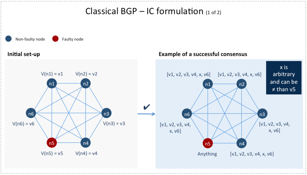
4) Agreement and validity criteria: Each non-faulty node in $\mathcal{P}$ computes an $n$ –vector whose $i^{th}$ entry is a value it calculates for the $i^{th}$ node such that:

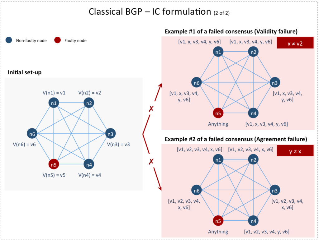
Agreement: All non-faulty nodes compute the same $n$ -vector $A = [v_{1}, .., v_{n}].$
Validity: If node $i$ is non-faulty and its private value is $v_{i}^{*},$ then the $i^{th}$ entry of $A$ computed by all non-faulty nodes is $v_{i}^{*}$ . In other words, $v_{i} = v_{i}^{*}.$

These consensus criteria are known as the Interactive Consistency (IC) formulation of the classical BGP [6]. Note that they do not require specifying which nodes are faulty. Furthermore, the elements of $A$ corresponding to faulty nodes may be arbitrary.

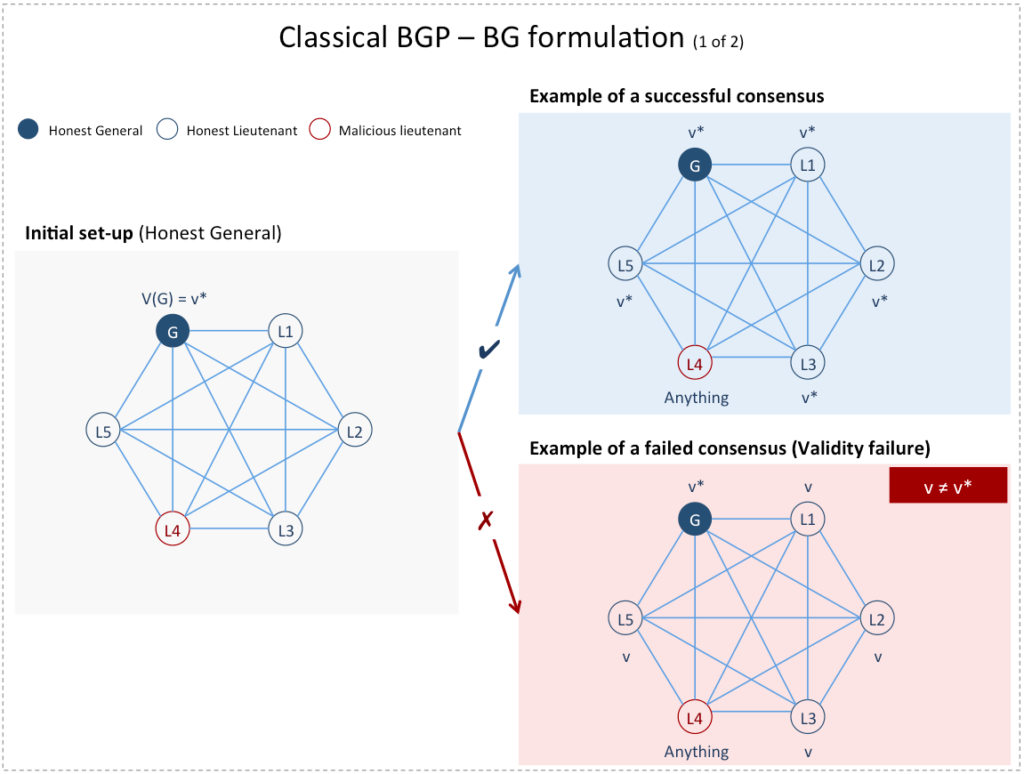
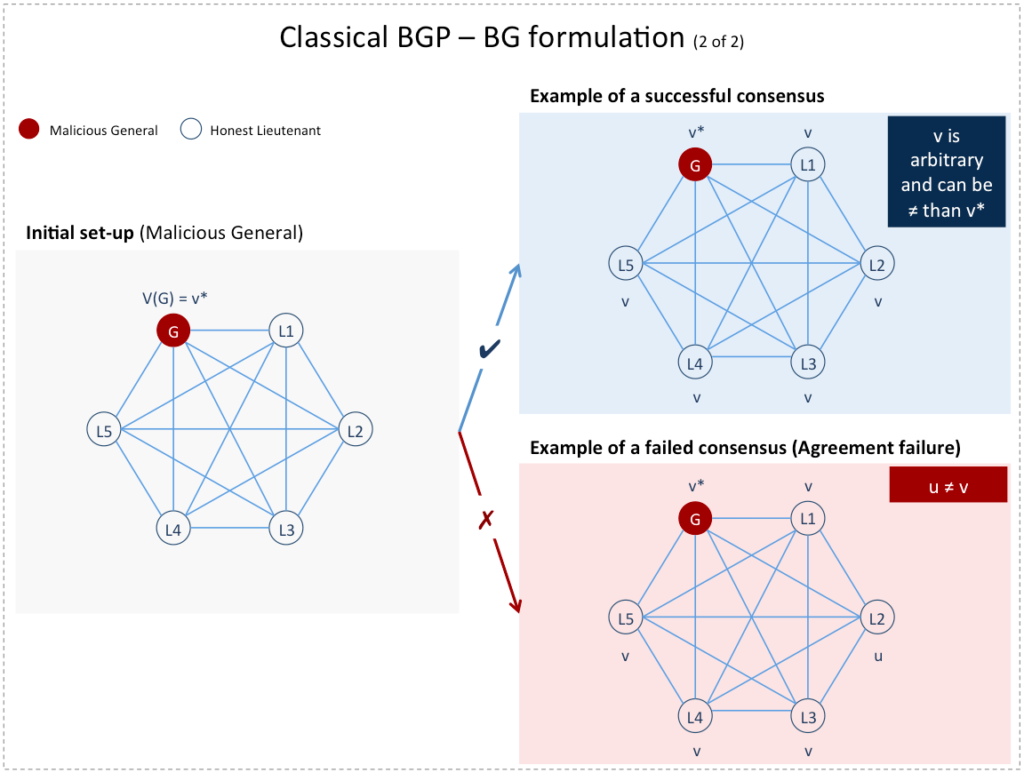
It turns out that the (IC) formulation can be equivalently expressed in two other ways: A Byzantine Generals (BG) formulation and a Consensus (C) one. The (BG) formulation introduced in [5] states that a General in the Byzantine army must send a value $v^{*}$ to his lieutenants such that:

Agreement: Honest lieutenants (i.e., non-faulty nodes) agree on a value $v.$
Validity: If the General is honest (i.e., source node is non-faulty), then $v = v^{*}.$

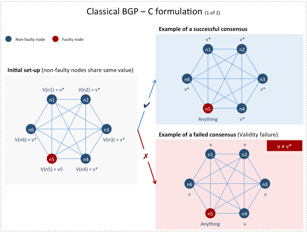
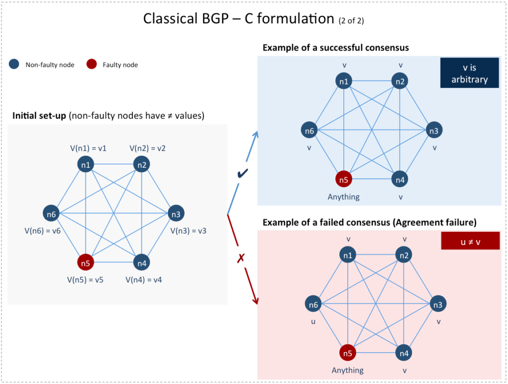
In the (C) formulation [3], each node is endowed with an initial value and the Agreement and Validity criteria become:

Agreement: All non-faulty nodes agree on the same single value $v.$
Validity: If all non-faulty nodes share the same initial value $v^{*},$ then their agreed upon value must be $v^{*}.$

BGP consensus formulations equivalence: In what follows we prove the equivalence of all three consensus formulations. More specifically, we show that an algorithm that can solve one of the problems can also be used to solve the other two. We denote by $F_{C},\ F_{BG},$ and $F_{IC}$ any algorithms that respectively solve the (C), (BG), and (IC) formulations of the classical BGP.

1) If there exists an $F_{C}$ then there exists an $F_{BG}$ : Without loss of generality, assume that the initial state of the (BG) formulation consists of general $i$ communicating his private value $v^{*}$ to his lieutenants. Conduct one round of communication and let $v_{j}^{*}$ be the value received by lieutenant $j.$ Set it as node $j$ ‘s initial value. Clearly, we also have that node $i$ ‘s initial value is $v_{i}^{*} = v^{*}.$ Now run $F_{C}$ on these initial states:

Since the Agreement criteria of $(C)$ ensures that all non-faulty nodes agree on the same single value $v,$ all honest lieutenants will certainly agree on the same value $v.$ This guarantees the Agreement criteria of (BG).
Now suppose that the general is honest (i.e., node $i$ is non-faulty). Then all non-faulty lieutenants will share the same initial value $v_{j}^{*} = v^{*}$ (i.e., the general’s private value). The Validity criteria of (C) would then ensure that their agreed upon value is $v^{*}.$ This proves that the Agreement criteria of (BG) is satisfied.

2) If there exists an $F_{BG}$ then there exists an $F_{IC}$ : For each non-faulty node $j \in \{1,\ ..,\ n\}$ let $v_{j}^{*}$ denote its private value and associate with it an $n$ -dimensional vector $A_{j}$ whose entries are all initialized to $0$ except for the $j^{th}$ entry whose value is set to $v_{j}^{*}.$ In other words, $A_{j}$ is initially set to $[0,\ ..,\ 0,\ v_{j}^{*},\ 0,\ ..,\ 0].$ For each node $i \in \{1,\ ..,\ n\}$ run $F_{BG}$ with node $i$ acting as general. Upon termination, update the $i^{th}$ entry of each $A_{j}$ with the resulting value computed by node $j$ :

If $i$ were a non-faulty node, then the (BG) Agreement and Validity criteria will ensure that all non-faulty lieutenants agree on the same value $v_{i}^{*}.$ As a result, the $i^{th}$ entry of each $A_{j}$ will be the same and equal to $v_{i}^{*}.$
If $i$ were a faulty node, then the (BG) Agreement criterion will ensure that all non-faulty lieutenants agree on some common value. As a result, the $i^{th}$ entry of each $A_{j}$ will be the same.

3) If there exists an $F_{IC}$ then there exists an $F_{C}$ : For each non-faulty node $j$ let $v_{j}^{*}$ denote its private value. Without loss of generality, suppose that the first $n-m$ nodes are non-faulty (i.e., $j \in \{1,\ ..,\ n-m\}).$ Run $F_{IC}$ to obtain an interactive consistecy vector $A = [v_{1}^{*},\ ..,\ v_{(n-m)}^{*},\ v_{(n-m+1)},\ ..,\ v_{n}].$ Note that the values $v_{k}$ ( $n-m < k \leq n$ ) are arbitrary as they correspond to faulty nodes. Let each non-faulty node pick the first entry of $A$ (i.e., $v_{1}^{*}$ ). This ensures that the Agreement and Validity criteria of (C) are met:

All non-faulty nodes agree on the same single value, namely $v_{1}^{*}.$
If all non-faulty nodes shared the same initial value $v^{*},$ then $v_{1}^{*} = v^{*}.$

An impossibility result for the classical BGP: It is not always possible to achieve consensus in a classical BGP setting. In [5] and [6], the authors showed that a necessary and sufficient condition for this to happen is for the total number $n$ of nodes to strictly exceed three times the number $m$ of faulty ones (i.e., $n > 3m$ ). We will lean on the (IC) formulation to demonstrate that this condition is necessary by showing that it is impossible to reach consensus if $n \leq 3m.$ We then rely on the equivalent (BG) formulation to prove that the condition is sufficient by describing an algorithm that achieves consensus whenever the condition is met [5].

We first start by formalizing the description of some of the system’s parameters introduced earlier. Recall that the underlying communication network is a digraph G with $n$ nodes, at most $m$ of which can be faulty. We succinctly denote this set-up by the triplet ( $G, n, m$ ). It is common to attach a processor $p_{i}$ to node $i$ and let $\mathcal{P}$ be the set $\{p_{1},\ ..,\ p_{n}\}.$ For all practical matters, the terms processor and node can be freely interchanged. Each processor has a private value (or initial state value) drawn from a set $\mathcal{V}.$ We let $v_{i}$ denote the private value of $p_{i}$

The objective is to devise an algorithm that can reach consensus irrespective of which processors are faulty, as long as there are at most $m$ of them. A particular instance of ( $G, n, m$ ) is called a system and is specified by:

The subset $\mathcal{N} \subset \mathcal{P}$ of non-faulty processors. Note that $|\mathcal{N}| \geq n-m.$
The behavior $\sigma$ of the processors as defined by the value that processor $p_{k}$ receives for processor $p_{j}$ when the transmission happens over some path in $\mathcal{P}.$ Clearly, if all processors were non-faulty, $p_{k}$ would receive the exact value sent by $p_{j}.$ Faulty processors on the other hand, may behave maliciously and their behavior may vary from one processor to another.

We denote the system associated with a given subset $\mathcal{N}$ and behavior $\sigma$ by $\xi_{(G,n,m),\ \mathcal{N},\ \sigma}.$ More formally, $\sigma$ is defined as the map:

$\sigma: \{\mathcal{P}\}^{*} \longrightarrow \mathcal{V}$

where $\{\mathcal{P}\}^{*}$ is the set of all non-empty strings over $\mathcal{P}$ (i.e., paths in $\mathcal{P}$ ) and $\mathcal{V}$ is an appropriate set of initial state values. We require that this map satisfies the following:

Initial state specification: $\sigma(p_{i}) = v_{i}.$ In other words, $\sigma$ maps each processor to its private value.
Behavior: For any path $p_{i_{1}}\ p_{i_{2}}\ p_{i_{3}}\ ..\ p_{i_{j-1}}\ p_{i_{j}}\ \in \mathcal{\{P\}^{*}},$ let $v \equiv \sigma(p_{i_{1}}\ p_{i_{2}}\ p_{i_{3}}\ ..\ p_{i_{j-1}}\ p_{i_{j}})$ be interpreted as

“ $p_{i_{2}}$ told $p_{i_{1}}$ that $p_{i_{3}}$ told $p_{i_{2}}$ that .. that $p_{i_{j}}$ told $p_{i_{j-1}}$ that its value was $v$ “.

Note that if $q \in \mathcal{N},$ then $\forall\ w \in \{\mathcal{P}\}^{*}$ and $\forall\ p \in \mathcal{P},$ we expect $\sigma(pqw)$ to be equal to $\sigma(qw).$ Indeed, by definition, a non-faulty $q$ must truthfully communicate whatever it receives. A behavior $\sigma$ that ensures this condition is said to be consistent with $\mathcal{N}.$

We rely on this formalism to define the notion of interactive consistency. Let $\mathcal{Z}_{(G,n,m)}$ be the space of all allowable systems on ( $G,n,m$ ) i.e., any system with:

A set of non-faulty processors $\mathcal{N}$ satisfying $|\mathcal{N}| \geq n-m,$ and;
A behavior $\sigma$ such that $\sigma$ is consistent with $\mathcal{N}$ .

In what follows, it is understood that a system is defined on ( $G,n,m$ ) and we write $\xi_{\mathcal{N}, \sigma}$ instead of $\xi_{(G,n,m),\ \mathcal{N}, \sigma}.$

Define the map $F_{IC}$ to be:

$F_{IC}: \mathcal{Z}_{(G,n,m)} \times \mathcal{P} \times \mathcal{P}\ \longrightarrow\ \mathcal{V}$

$(\xi_{\mathcal{N}, \sigma}\ ,\ p_{i},\ p_{k}) \longrightarrow F_{IC}\ ({\xi_{\mathcal{N}, \sigma}}\ ,\ p_{i},\ p_{k})$

where for an allowable system $\xi_{\mathcal{N}, \sigma},$ the output corresponds to the value of processor $p_{k}$ computed by processor $p_{i}$ in the (IC) formulation. If $i = k,$ the output is taken to be $p_{i}$ ‘s private value. The consistency vector computed by $p_{i}$ is then the $n$ -dimensional vector:

$A = [F_{IC}\ ({\xi_{\mathcal{N}, \sigma}}\ ,\ p_{i},\ p_{1}),\ ..,\ F_{IC}\ ({\xi_{\mathcal{N}, \sigma}}\ ,\ p_{i},\ p_{n}],$

Note that $F_{IC}\ ({\xi_{\mathcal{N}, \sigma}}\ ,\ p_{i},\ p_{k})$ is calculated based on one or more pieces of information available to processor $p_{i}.$ Each such piece of information is received by $p_{i}$ over some path in $\{\mathcal{P}\}^{*}$ and is hence of the form $\sigma(p_{i}\ r_{1}\ r_{2}\ .. )$ where $r_{1}, r_{2}, .., \in \mathcal{P}.$ We denote the restriction of $\sigma$ to paths in $\{\mathcal{P}\}^{*}$ starting with $p_{i}$ by $\sigma_{p_{i}}.$

We say that $F_{IC}$ solves the (IC) formulation if $\forall\ \xi_{\mathcal{N}, \sigma} \in \mathcal{Z}_{(G,n,m)},$ the following consensus conditions hold:

1) Agreement condition: $\forall\ p_{i},\ p_{j} \in \mathcal{N},\ \forall\ p_{k} \in \mathcal{P},$

$F_{IC}\ ({\xi_{\mathcal{N}, \sigma}}\ ,\ p_{i},\ p_{k}) = F_{IC}\ ({\xi_{\mathcal{N}, \sigma}}\ ,\ p_{j},\ p_{k}).$

Intuitively, this condition requires that any two non-faulty processors share the same consistency vector. This is the Agreement criterion of the (IC) formulation.

2) Validity condition: $\forall\ p_{i},\ p_{k} \in \mathcal{N},$

$F_{IC}\ ({\xi_{\mathcal{N}, \sigma}}\ ,\ p_{i},\ p_{k}) = \sigma(p_{k}).$

Intuitively, this condition requires that the entry corresponding to a non-faulty processor $p_{k}$ in the consistency vector computed by a non-faulty processor $p_{i}$ be $p_{k}$ ‘s private value. This is the Validity criterion of the IC formulation.

We can now formally state and prove the classical BGP’s impossibility result:

$|\mathcal{V}| \geq 2$ and $n \leq 3m\ \implies\ \nexists\ F_{IC}$ that solves the (IC) formulation of BGP.

The proof is a reductio ad absurdum. Suppose that given $|\mathcal{V}| \geq 2$ and $n \leq 3m,$ one were able to find such an $F_{IC}$ (i.e., an $F_{IC}$ that achieves consensus on any allowable system $\xi_{\mathcal{N}, \sigma} \in \mathcal{Z}_{(G,n,m)}).$ Our objective is to construct three systems whose coexistence would contradict the Agreement criterion needed for $F_{IC}$ to be an acceptable solution.

Since $n \leq 3m,$ one can partition $\mathcal{P}$ into three non-empty subsets $\mathcal{A}, \mathcal{B},$ and $\mathcal{C}$ such that

max( $|\mathcal{A}|, |\mathcal{B}|, |\mathcal{C}|$ ) $\leq m.$

Furthermore, since $|\mathcal{V}| \geq 2,\ \exists\ v, v' \in \mathcal{V}$ such that $v \neq v'.$

Consider the system $\xi_{\mathcal{N}, \alpha}$ where $\mathcal{N} \equiv \mathcal{B} \cup \mathcal{C},$ and $\alpha$ some behavior consistent with $\mathcal{B} \cup \mathcal{C}.$ Then $\xi_{(\mathcal{B} \cup \mathcal{C}), \alpha}\ \in\ \mathcal{Z}_{(G,n,m)}$ since $|\mathcal{B} \cup \mathcal{C}| = |\mathcal{P} - \mathcal{A}| \geq n-m.$ Similarly, we can consider the two other systems $\xi_{(\mathcal{A} \cup \mathcal{C}), \beta}$ and $\xi_{(\mathcal{A} \cup \mathcal{B}), \gamma}$ in $\mathcal{Z}_{(G,n,m)}$ where $\beta$ is some behavior consistent with $\mathcal{A} \cup \mathcal{C}$ and $\gamma$ with $\mathcal{A} \cup \mathcal{B}.$

Suppose that in addition to being respectively consistent with $\mathcal{B} \cup \mathcal{C},\ \mathcal{A} \cup \mathcal{C},$ and $\mathcal{A} \cup \mathcal{B}$ , behaviors $\alpha,\ \beta,$ and $\gamma$ also satisfied the following constraints:

For any $a \in \mathcal{A},\ \beta$ and $\gamma$ are indistinguishable, i.e., $\beta_{a} = \gamma_{a}$ (this refers to the restriction of a behavior to paths in $\{\mathcal{P}\}^{*}$ starting with $a).$
$\forall\ b \in \mathcal{B},$ behaviors $\alpha$ and $\gamma$ are indistinguishable, i.e., $\alpha_{b} = \gamma_{b}.$
$\forall\ c \in \mathcal{C},$ $\alpha(c) \neq \beta(c).$

We could then reach the desired contradiction as follows:

$F_{IC}\ ( \xi_{(\mathcal{A} \cup \mathcal{B}), \gamma}\ ,\ a,\ c)$ solely depends on $\gamma_{a}.$ And since $\gamma_{a} = \beta_{a},$ it is equal to $F_{IC}\ ( \xi_{(\mathcal{A} \cup \mathcal{C}), \beta}\ ,\ a,\ c).$
$F_{IC}\ ( \xi_{(\mathcal{A} \cup \mathcal{C}), \beta}\ ,\ a,\ c)\ =\ \beta(c)$ by the Validity criterion of $(IC).$
$\beta(c) \neq \alpha(c)$ by design of the behaviors $\beta$ and $\alpha.$
$\alpha(c)\ =\ F_{IC}\ ( \xi_{(\mathcal{B} \cup \mathcal{C}), \alpha}\ ,\ b,\ c)$ by the Validity criterion of $(IC).$
$F_{IC}\ ( \xi_{(\mathcal{B} \cup \mathcal{C}), \alpha}\ ,\ b,\ c)$ solely depends on $\alpha_{b}.$ And since $\alpha_{b} = \gamma_{b},$ it is equal to $F_{IC}\ ( \xi_{(\mathcal{A} \cup \mathcal{B}), \gamma}\ ,\ b,\ c).$
As a result, $F_{IC}\ ( \xi_{(\mathcal{A} \cup \mathcal{B}), \gamma}\ ,\ a,\ c)\ \neq\ F_{IC}\ ( \xi_{(\mathcal{A} \cup \mathcal{B}), \gamma}\ ,\ b,\ c).$ This contradicts the Agreement criterion of (IC) since $\gamma$ is consistent with $\mathcal{A} \cup \mathcal{B},$ and $a,\ b\ \in \mathcal{A} \cup \mathcal{B}.$

Consequently, all that is needed to complete the proof is to construct $\alpha,\ \beta,$ and $\gamma$ satisfying these constraints. Note that elements of $\{\mathcal{P}\}^{*}$ can be of three types:

1) Strings $w$ that don’t end with a processor in $\mathcal{C}.$ In this case, let

$\alpha(w)\ =\ \beta(w)\ =\ \gamma(w)\ =\ v.$

2) Strings of length 1 or 2 that end with a processor in $\mathcal{C}.\ \forall\ a \in \mathcal{A},$ $b \in \mathcal{B},\ c \in \mathcal{C},$ let

$\alpha(c) = \alpha(a\ c) = \alpha(b\ c) = \alpha(c\ c) = v$

$\beta(c) = \beta(a\ c) = \beta(b\ c) = \beta(c\ c) = v'$

$\gamma(c) = \gamma(b\ c) = \gamma(c\ c) = v$ and $\gamma(a\ c) = v'$

3) Strings of length greater than 2 that end with a processor in $\mathcal{C}.$ For any string $w$ ending with a processor in $\mathcal{C},$ and $\forall\ a \in \mathcal{A},\ b \in \mathcal{B},\ c \in \mathcal{C},$ $p \in \mathcal{P},$ let

$\alpha(p\ a\ w) = \beta(a\ w),\ \alpha(p\ b\ w) = \alpha(b\ w),$ and $\alpha(p\ c\ w) = \alpha(c\ w)$

$\beta(p\ a\ w) = \beta(a\ w),\ \beta(p\ b\ w) = \alpha(b\ w),$ and $\beta(p\ c\ w) = \beta(c\ w)$

$\gamma(p\ a\ w) = \gamma(a\ w),\ \gamma(p\ b\ w) = \gamma(b\ w),\ \gamma(a\ c\ w) = \beta(c\ w),$ $\gamma(b\ c\ w) = \alpha(c\ w),$ and $\gamma(c\ c\ w) = \gamma(c\ w)$

Note that by defining the action of the various behaviors on a string of length $l \geq 2$ in terms of the action of one of these maps on a string of length $l-1,$ one can easily compute the actual values recursively as they have been previously defined for the cases $l = 1$ and $l = 2.$

Clearly, behavior $\alpha$ is consistent with $\mathcal{B} \cup \mathcal{C}.$ Indeed, $\forall\ q \in \mathcal{B} \cup \mathcal{C}$ (i.e., $q$ is of the form $b$ or $c$ ), and $\forall\ p \in \mathcal{P}$ and $w \in \{\mathcal{P}\}^{*},$ we have $\alpha(p\ b\ w) = \alpha(b\ w)$ and $\alpha(p\ c\ w) = \alpha(c\ w).$

Similarly, behavior $\beta$ is consistent with $\mathcal{A} \cup \mathcal{C}$ since $\forall\ q \in \mathcal{A} \cup \mathcal{C}$ (i.e., $q$ is of the form $a$ or $c$ ), and $\forall\ p \in \mathcal{P}$ and $w \in \{\mathcal{P}\}^{*}$ we have $\beta(p\ a\ w) = \beta(a\ w)$ and $\beta(p\ c\ w) = \beta(c\ w).$

Finally, behavior $\gamma$ is consistent with $\mathcal{A} \cup \mathcal{B}$ since $\forall\ q \in \mathcal{A} \cup \mathcal{B}$ (i.e., $q$ is of the form $a$ or $b$ ), and $\forall\ p \in \mathcal{P}$ and $w \in \{\mathcal{P}\}^{*},$ we have $\gamma(p\ a\ w) = \gamma(a\ w)$ and $\gamma(p\ b\ w) = \gamma(b\ w).$

Next we show that $\forall\ a \in \mathcal{A},$ behaviors $\beta$ and $\gamma$ are indistinguishable (i.e., $\beta_{a} = \gamma_{a},$ ) and $\forall\ b \in \mathcal{B},$ behaviors $\alpha$ and $\gamma$ are indistinguishable (i.e., $\alpha_{b} = \gamma_{b}$ ).

First, note that $\forall\ w \in \{\mathcal{P}\}^{*}$ not ending in a processor in $\mathcal{C},$ the construction mandates that $\alpha(w) = \beta(w) = \gamma(w) = v.$ In particular this holds true for such strings that start with a processor in $\mathcal{A}$ and so $\beta_{a} = \gamma_{a} = v.$ In addition, this holds true for such strings that start with a processor in $\mathcal{B}$ and so $\alpha_{b} = \gamma_{b} = v.$

To show it for strings $w \in \{\mathcal{P}\}^{*}$ ending in a processor in $\mathcal{C},$ we proceed by induction on the length of $w.$ If $w$ is of length 1, i.e., $w \in \mathcal{C},$ the construction mandates that $\beta(a\ c) = \gamma(a\ c) = v'$ and so $\beta_{a}$ and $\gamma_{a}$ are indistinguishable over elements of $\mathcal{C}.$ Similarly, the construction mandates that $\alpha(b\ c) = \gamma(b\ c) = v$ and so $\alpha_{b}$ and $\gamma_{b}$ are indistinguishable over elements of $\mathcal{C}.$

Now suppose that the result holds true for strings $w \in \{\mathcal{P}\}^{*}$ of length $l > 1$ that end in a processor in $\mathcal{C}.$ Relevant strings of length $l+1$ must be of the form $aw,\ bw$ or $cw$ ( $a \in \mathcal{A},\ b \in \mathcal{B},\ c \in \mathcal{C}$ ). We must show that:

$\beta(a\ a\ w) = \gamma(a\ a\ w),\ \beta(a\ b\ w) = \gamma(a\ b\ w),$ and $\beta(a\ c\ w) = \gamma(a\ c\ w)$
$\alpha(b\ a\ w) = \gamma(b\ a\ w),\ \alpha(b\ b\ w) = \gamma(b\ b\ w),$ and $\alpha(b\ c\ w) = \gamma(b\ c\ w).$

We will show it only for 1. as 2. can be done in exactly the same way:

$\beta(a\ a\ w) = \beta(a\ w)$ (by construction), which is equal to $\gamma(a\ w)$ (by induction), which in turn is equal to $\gamma(a\ a\ w)$ (by construction).
$\beta(a\ b\ w) = \alpha(b\ w)$ (by construction), which is equal to $\gamma(b\ w)$ (by induction), which in turn is equal to $\gamma(a\ b\ w)$ (by construction).
$\beta(a\ c\ w) = \beta(c\ w)$ (by construction), which is equal to $\gamma(a\ c\ w)$ (by construction).

Here is a summary of the three systems for the case $n=3$ and $m=1:$

Classical BGP consensus - Impossibility result

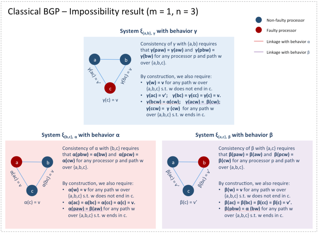
The intuition is as follows:

From the point of view of processor $a,$ systems $\xi_{\{a,b\}, \gamma}$ and $\xi_{\{a,c\}, \beta}$ are indistinguishable because $\gamma$ and $\beta$ are identical when restricted to strings starting with $a.$ As a result, $a$ cannot tell whether $c$ is faulty (i.e., system $\xi_{\{a,b\}, \gamma}$ is applicable) or $b$ is (i.e., system $\xi_{\{a,c\}, \beta}$ is applicable). In order not to violate the Validity condition in $\xi_{\{a,c\}, \beta},\ a$ is then forced to register for $c$ the value $\beta(c) = v'.$
Similarly, from the point of view of processor $b,$ systems $\xi_{\{a,b\}, \gamma}$ and $\xi_{\{b,c\}, \alpha}$ are indistinguishable because $\gamma$ and $\alpha$ are identical when restricted to strings starting with $b.$ As a result, $b$ cannot tell whether $c$ is faulty (i.e., system $\xi_{\{a,b\}, \gamma}$ is applicable) or $a$ is (i.e., system $\xi_{\{b,c\}, \alpha}$ is applicable). In order not to violate the Validity condition in $\xi_{\{b,c\}, \alpha},\ b$ is then forced to register for $c$ the value $\alpha(c) = v.$
But in order not to violate the Agreement condition in system $\xi_{\{a,b\}, \gamma},$ processors $a$ and $b$ must both register the same value for processor $c.$ However, this is not the case since $a$ registered $v'$ while $b$ registered $v.$

Note that this proof fails if $n > 3m.$ This is because any 3-subset partition $(\mathcal{A},\ \mathcal{B},\ \mathcal{C})$ of $\mathcal{P}$ would have at least one subset $\mathcal{A}$ with $|\mathcal{A}| > m.$ This would cause system $\xi_{(\mathcal{B} \cup \mathcal{C}), \alpha}$ to be not allowable (i.e., $\notin\ \mathcal{Z}_{(G,n,m)}$ ).

Solving the classical BGP for $n > 3m$ : We now show that the necessary condition $n > 3m$ is also sufficient. We do so by describing an algorithm $F_{BG}$ that achieves consensus in the (BG) formulation.

For a given allowable system $\xi_{\mathcal{N}, \sigma}$ in $\mathcal{Z}_{(G,n,m)},$ and processor $p_{k} \in \mathcal{P}$ acting as general, we make explicit the dependence of $F_{BG}$ on $m,\ p_{k}$ and $\mathcal{P}$ and write $F_{BG}^{(m,\ p_{k},\ \mathcal{P})}.$ We define the map $F_{BG}^{(m,\ p_{k},\ \mathcal{P})}$ to be:

$F_{BG}^{(m,\ p_{k},\ \mathcal{P})}:\ \mathcal{Z}_{(G,n,m)} \times \mathcal{P} \times \{p_{k}\}\ \longrightarrow\ \mathcal{V}$

$(\xi_{\mathcal{N}, \sigma}\ ,\ p_{i},\ p_{k}) \longrightarrow F_{BG}^{(m,\ p_{k},\ \mathcal{P})}\ ({\xi_{\mathcal{N}, \sigma}}\ ,\ p_{i},\ p_{k})$

where the output corresponds to the value that processor $p_{i}$ computes for $p_{k}.$ We say that $F_{BG}^{(m,\ p_{k},\ \mathcal{P})}$ solves the (BG) formulation if $\forall\ \xi_{\mathcal{N}, \sigma} \in \mathcal{Z}_{(G,n,m)}$ the following consensus conditions hold:

1. Agreement: $\forall\ p_{i},\ p_{j} \in \mathcal{N},$

$F_{BG}^{(m,\ p_{k},\ \mathcal{P})}\ ({\xi_{\mathcal{N}, \sigma}}\ ,\ p_{i},\ p_{k}) = F_{BG}^{(m,\ p_{k},\ \mathcal{P})}\ ({\xi_{\mathcal{N}, \sigma}}\ ,\ p_{j},\ p_{k}).$

Intuitively, non-faulty lieutenants must compute the same value for general $p_{k}$ .

2. Validity: If $p_{k} \in \mathcal{N},$ then $\forall\ p_{i} \in \mathcal{N},$

$F_{BG}^{(m,\ p_{k},\ \mathcal{P})}\ ({\xi_{\mathcal{N}, \sigma}}\ ,\ p_{i},\ p_{k}) = \sigma(p_{k}).$

Intuitively, this requires that the value that a non-faulty lieutenant $p_{i}$ computes for a non-faulty general $p_{k}$ be $p_{k}$ ‘s private value.

To devise such a map, we introduce a recursive algorithm $\mathcal{A}(r,\ q_{k},\ \mathcal{S})$ over $\xi_{\mathcal{N}, \sigma}$ that takes three inputs: a subset $\mathcal{S} \equiv \{q_{1},\ ..,\ q_{s}\}\ \subseteq\ \mathcal{P} \equiv \{p_{1},\ ..,\ p_{n}\},$ a processor $q_{k} \in \mathcal{S}$ and an iteration variable $r$ such that $0 \leq r \leq s-1:$

Base case $\mathcal{A}(0,\ q_{k},\ \mathcal{S}):$ When $r$ is 0, processor $q_{k}$ sends its value to every other processor $q_{i} \in \mathcal{S}$ who receives value $\sigma(q_{i}\ q_{k})$ and attributes it to $q_{k}.$

General case $\mathcal{A}(r,\ q_{k},\ \mathcal{S})$ for $r > 0:$

i) Processor $q_{k}$ sends its value to every other $q_{i} \in \mathcal{S}.$

ii) Processor $q_{i}$ receives value $v_{ik} \equiv \sigma(q_{i}\ q_{k}).$ A new instance of algorithm $\mathcal{A}$ is then executed for each $q_{i}$ with an iteration counter set to $r-1$ and a processor set $\mathcal{S}-\{q_{k}\}.$ Each such iteration sends $v_{ik}$ to the remaining processors $q_{j},\ j\ \in\ \{1,\ ..,\ s\},\ j \notin\ \{k,\ i\}.$ This step runs an instance of $\mathcal{A}(r-1,\ q_{i},\ \mathcal{S}-\{q_{k}\})$ for each $q_{i} \in \mathcal{S} - \{q_{k}\}$ totaling $(s-1)$ instances.

iii) $\forall\ i, j \in \{1,\ ..,\ s\},\ i,j \notin \{k\},\ i \neq j,$ let $v_{ij} \equiv \sigma(q_{i}\ q_{j}\ q_{k})$ denote the value that $q_{i}$ computed for $q_{j}$ under algorithm $\mathcal{A}(r-1,\ q_{j},\ \mathcal{S}-\{q_{k}\})$ in step ii). Subsequently, $q_{i}$ computes the following value and assigns it to $q_{k}:$

$w_{ik} \equiv majority\ (v_{i1},\ ..,\ v_{ij},\ ..,\ v_{in}),\ \forall j \in \{1,\ ..,\ n\},\ j \neq i$

We can represent the above logic in pseudo-code as follows:

Define $\mathcal{A}(r, q_{k}, \mathcal{S}):$

$\{$

If $r$ is equal to $0:$

$\{$

For each $q_{i} \in \mathcal{S},\ i \neq k,$ do the following:

$\{$

$q_{i}$ receives $\sigma(q_{i}\ q_{k})$

$q_{i}$ assigns the value $w_{ik} \equiv \sigma(q_{i}\ q_{k})$ to $q_{k}$

$\}$

Else, if $r>0$ :

$\{$

For each $q_{i} \in \mathcal{S},\ i \neq k,$ do the following:

$\{$

$q_{i}$ receives $v_{ik} \equiv \sigma(q_{i}\ q_{k})$ and sets it as its private value

Run $\mathcal{A}(r-1,\ q_{i},\ \mathcal{S} - \{q_{k}\})$ and store the resulting $(s-2)$ vector $[v_{1i},\ ..,\ v_{ji},\ ..,\ v_{si}],$ where $v_{ji}$ denotes the value that $q_{j}$ computed for $q_{i},$ and where $j \in \{1,\ ..,\ s\},\ j \notin \{i, k\}$

$\}$

For each $q_{i} \in \mathcal{S},\ i \neq k,\ q_{i}$ does the following:

$\{$

Assign $w_{ik} \equiv majority\ (v_{i1},\ ..,\ v_{ik},\ ..,\ v_{ij},\ ..,\ v_{is})$ to $q_{k}$ where the index $j \in \{1,\ ..,\ s\},\ j \neq i$

$\}$

Return the $(s-1)$ vector $[w_{1k},\ ..,\ w_{jk},\ ..,\ w_{sk}],$ where $j \in \{1,\ ..,\ s\},\ j \neq k$

$\}$

Algorithm $\mathcal{A}(r,\ q_{k},\ \mathcal{S})$ invokes $(s-1)$ algorithms of order $(r-1)$ namely, $\mathcal{A}(r-1,\ q_{i},\ \mathcal{S}-\{q_{k}\}),$ $\ i\ \in\ \{1,\ ..,\ s\},$ $i \neq k$ . Similarly, each algorithm of order $(r-1)$ invokes $(s-2)$ others of order $(r-2).$ The lowest order ones have $r=0$ and are called $(s-1)\ ...\ (s-r)$ times. Finally, each algorithm of order 0 sends $(s-r-1)$ messages, resulting in a total of $(s-1)\ ...\ (s-r)(s-r-1)$ messages and a complexity of $\mathcal{O}(s^{(r+1)}).$

$\forall i \in \{1,\ ..,\ n\},\ i \neq k,$ we now define the map $F_{BG}^{(m, p_{k}, \mathcal{P})}$ as follows:

$F_{BG}^{(m, p_{k}, \mathcal{P})}\ ({\xi_{\mathcal{N}, \sigma}}\ ,\ p_{i},\ p_{k}) \equiv w_{ik}$

where $w_{ik}$ is the appropriate component of the $(n-1)$ vector returned by $\mathcal{A}(m,\ p_{k},\ \mathcal{P})$ with an iteration count set to $m$ (the maximal number of faulty processors allowed).

We claim that this map solves the (BG) formulation of the classical BGP whenever $m > 3n.$ Before we prove its correctness, we look at two clarifying examples (we will drop the $\mathcal{P}$ superscript for ease of notation)

Example 1, $(m,n) = (1,4):$ Let $\mathcal{N} = \{p_{1}, p_{2}, p_{3}\}$ and $p_{4}$ be faulty. There are two cases depending on whether the general is faulty or not. We will refer to processors by their indices and enclose received values in brackets and computed values in parentheses:

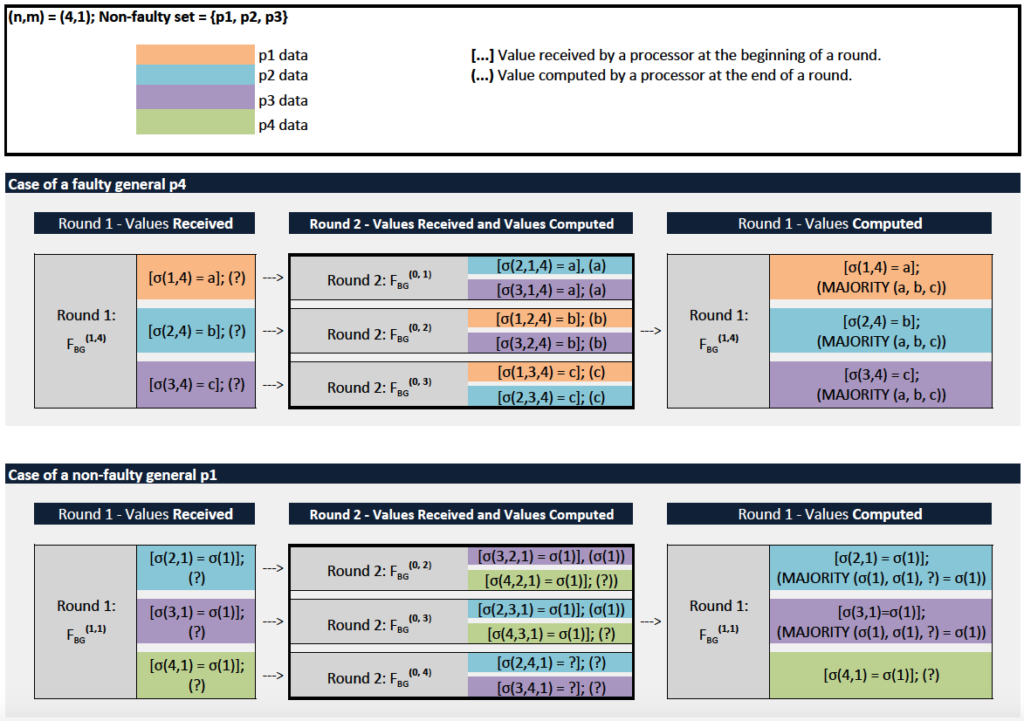
We describe the case of a faulty general (the other one can be analyzed similarly):

Algorithm $F_{BG}^{(1, 4)}$ is invoked and $p_{4}$ sends its value to every lieutenant $i \in \{1,2,3\}.$
Lieutenant $i$ receives value $v_{i4} \equiv \sigma(i\ 4).$ Let $v_{14} = a,\ v_{24} = b,$ and $v_{34} = c.$ Subsequently, each $i \in \{1,2,3\}$ acts as general and runs a new instance of algorithm $F_{BG}^{(0,\ i)}$ to send $v_{i4}$ to the remaining two lieutenants. More specifically:

- Under $F_{BG}^{(0,\ 1)},$ $p_{1}$ sends $v_{21} = \sigma(2\ 1\ 4) = a$ to lieutenant $2$ and $v_{31} = \sigma(3\ 1\ 4) = a$ to lieutenant $3.$
- Under $F_{BG}^{(0,\ 2)}$ $p_{2}$ sends $v_{12} = \sigma(1\ 2\ 4) = b$ to lieutenant $1$ and $v_{32} = \sigma(3\ 2\ 4) = b$ to lieutenant $3.$
- Finally, under $F_{BG}^{(0,\ 3)}$ $p_{3}$ sends $v_{13} = \sigma(1\ 3\ 4) = c$ to lieutenants $1$ and $v_{23} = \sigma(2\ 3\ 4) = c$ to lieutenant $2.$
Since the algorithm is running instances with $m=0,$ it must be that lieutenants $2$ and $3$ compute a value equals to $a$ under $F_{BG}^{(0,\ 1)}.$ Similarly, lieutenants $1$ and $3$ compute $b$ under $F_{BG}^{(0,\ 2)},$ while lieutenants $1$ and $2$ compute $c$ under $F_{BG}^{(0,\ 3)}.$
Finally, the value that lieutenants $1, 2$ and $3$ computes for $p_{4}$ under $F_{BG}^{(1,\ 4)}$ is equal to:

$majority\ (v_{14}, v_{12}, v_{13})\ =\ majority\ (a, b, c)$

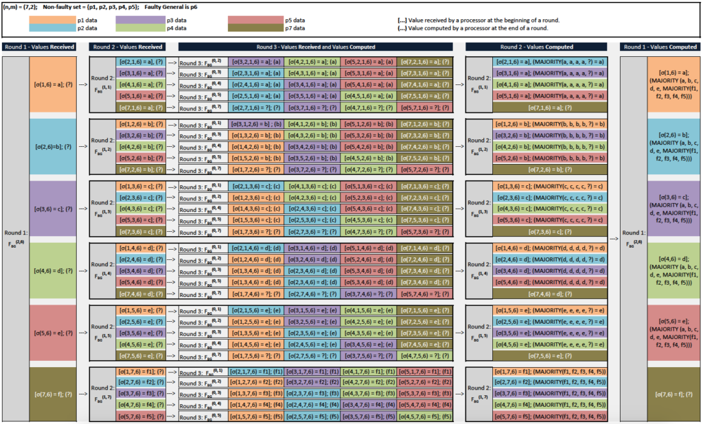
Example 2, $(m,n) = (2,7):$ Let $\mathcal{N} = \{1, 2, 3, 4, 5\}$ and $\{6,7\}$ be faulty. Here too, there are two cases depending on whether the general is faulty or not. We treat the case of a faulty general $p_{6}$ (the other case can be analyzed similarly) and follow the convention of enclosing received values in brackets and computed values in parentheses:

Algorithm $F_{BG}^{(2, 6)}$ is invoked and processor $6$ sends its value to every lieutenant $i \in \{1,2,3,4,5,7\}.$
Lieutenant $i$ receives value $v_{i6} = \sigma(i\ 6).$ Let $v_{16} = \sigma(1\ 6) = a,$ $v_{26} = \sigma(2\ 6) = b,$ $v_{36} = \sigma(3\ 6) = c,$ $v_{46} = \sigma(4\ 6) = d,$ $v_{56} = \sigma(5\ 6) = e,$ and $v_{76} = \sigma(7\ 6) = f.$ Subsequently, each $i \in \{1,2,3,4,5,7\}$ acts as general and runs $F_{BG}^{(1,\ i)}$ to send $v_{i6}$ to the other five lieutenants.
The next step is to compute the action of $F_{BG}^{(1,\ i)}.$ We illustrate it for $F_{BG}^{(1,\ 3)}$ where processor $3$ acts as general and sends its value $v_{36} = \sigma(3\ 6) = c$ to the remaining five lieutenants $\{1,2,4,5,7\}$ . In this case, lieutenant $j$ receives $v_{j3} = \sigma(j\ 3\ 6) = c,\ \forall j \in \{1,2,4,5,7\}.$ Subsequently, each $j \in \{1,2,4,5,7\}$ acts as general and runs a new instance of algorithm $F_{BG}^{(0,\ j)}$ to send $v_{j3}$ to the remaining four lieutenants:

- Under $F_{BG}^{(0,\ 1)},$ processor $1$ acts as general and sends its value $\sigma(1\ 3\ 6) = c$ to lieutenants $\{2,4,5,7\}.$ Lieutenant $k$ receives $\sigma(k\ 1\ 3\ 6) = c,\ \forall k \in \{2,4,5,7\}.$
- Under $F_{BG}^{(0,\ 2)},$ processor $2$ acts as general and sends its value $\sigma(2\ 3\ 6) = c$ to lieutenants $\{1,4,5,7\}.$ Lieutenant $k$ receives $\sigma(k\ 2\ 3\ 6) = c,\ \forall k \in \{1,4,5,7\}.$
- Under $F_{BG}^{(0,\ 4)},$ processor $4$ acts as general and sends its value $\sigma(4\ 3\ 6) = c$ to lieutenants $\{1,2,5,7\}.$ Lieutenant $k$ receives $\sigma(k\ 4\ 3\ 6) = c,\ \forall k \in \{1,2,5,7\}.$
- Under $F_{BG}^{(0,\ 5)},$ processor $5$ acts as general and sends its value $\sigma(5\ 3\ 6) = c$ to lieutenants $\{1,2,4,7\}.$ Lieutenant $k$ receives $\sigma(k\ 5\ 3\ 6) = c,\ \forall k \in \{1,2,4,7\}.$
- Under $F_{BG}^{(0,\ 7)},$ faulty processor $p_{7}$ acts as general and sends some unknown value(s) to lieutenants $\{1,2,4,5\}.$ Each lieutenant $k \in \{1,2,4,5\}$ receives an unknown value $\sigma(k\ 7\ 3\ 6)$ that we denote by a question mark (?).
Since $m=0,$ each received values also serves as the computed value that the relevant processor attributes to $p_{6}.$ We can now compute the value that the non-faulty lieutenants $1, 2, 4$ and $5$ compute for $p_{6}$ under $F_{BG}^{(1,\ 3)}:$

- Lieutenant $1$ computes:

$majority\ (\sigma(1\ 3\ 6), \sigma(1\ 2\ 3\ 6), \sigma(1\ 4\ 3\ 6),$

$\sigma(1\ 5\ 3\ 6), \sigma(1\ 7\ 3\ 6))\ =\ majority\ (c, c, c, c, ?)\ =\ c$

- Lieutenant $2$ computes:

$majority\ (\sigma(2\ 3\ 6), \sigma(2\ 1\ 3\ 6), \sigma(2\ 4\ 3\ 6),$

$\sigma(2\ 5\ 3\ 6), \sigma(2\ 7\ 3\ 6))\ =\ majority\ (c, c, c, c, ?)\ =\ c$

- Lieutenant $4$ computes:

$majority\ (\sigma(4\ 3\ 6), \sigma(4\ 1\ 3\ 6), \sigma(4\ 2\ 3\ 6),$

$\sigma(4\ 5\ 3\ 6), \sigma(4\ 7\ 3\ 6))\ =\ majority\ (c, c, c, c, ?)\ =\ c$

- Lieutenant $5$ computes:

$majority\ (\sigma(5\ 3\ 6), \sigma(5\ 1\ 3\ 6), \sigma(5\ 2\ 3\ 6),$

$\sigma(5\ 4\ 3\ 6), \sigma(5\ 7\ 3\ 6))\ =\ majority\ (c, c, c, c, ?)\ =\ c$

Similarly, one can evaluate $F_{BG}^{(1,\ i)},\ i \in \{1, 2, 4, 5, 7\}:$
- For $F_{BG}^{(1,\ 1)},$ we find that the values that the non-faulty lieutenants $2, 3, 4$ and $5$ compute for $p_{6}$ are all equal to $majority\ (a, a, a, a, ?)\ =\ a.$
- For $F_{BG}^{(1,\ 2)},$ we find that the values that the non-faulty lieutenants $1, 3, 4$ and $5$ compute for $p_{6}$ are all equal to $majority\ (b, b, b, b, ?)\ =\ b.$
- For $F_{BG}^{(1,\ 4)},$ we find that the values that the non-faulty lieutenants $1, 2, 3$ and $5$ compute for $p_{6}$ are all equal to $majority\ (d, d, d, d, ?)\ =\ d.$
- For $F_{BG}^{(1,\ 5)},$ we find that the values that the non-faulty lieutenants $1, 2, 3$ and $4$ compute for $p_{6}$ are all equal to $majority\ (e, e, e, e, ?)\ =\ e.$
- For $F_{BG}^{(1,\ 7)},$ we find that the values that the non-faulty lieutenants $1, 2, 3, 4$ and $5$ compute for $p_{6}$ are all equal to $majority\ (f1, f2, f3, f4, f5)$ where $f_{s},\ s \in \{1,2,3,4,5\}$ denotes the value $\sigma(s\ 7\ 6)$ that $p_{7}$ communicates to processor $s$ under $F_{BG}^{(1,\ 7)}.$ These values may be different from each other since $p_{7}$ is faulty.

Finally, the value that the non-faulty lieutenants compute for under are as follows:
- Lieutenant $1$ computes $majority\ (a, b, c, d, e,\ majority\ (f1, f2, f3, f4, f5)\ )$
- Lieutenant $2$ computes $majority\ (a, b, c, d, e,\ majority\ (f1, f2, f3, f4, f5)\ )$
- Lieutenant $3$ computes $majority\ (a, b, c, d, e,\ majority\ (f1, f2, f3, f4, f5)\ )$
- Lieutenant $4$ computes: $majority\ (a, b, c, d, e,\ majority\ (f1, f2, f3, f4, f5)\ )$

Proof of the algorithm’s correctness: We wrap up this section with a correctness proof for the aforementioned algorithm whenever $n > 3m$ .

Let $\mathcal{P} \equiv \{p_{1},\ p_{2},\ ..,\ p_{n}\}$ be a set of $n$ processors, with $p_{k}$ acting as general for some $k \in \{1,\ ..,\ n\}$ . Furthermore, assume that at most $m$ out of $n$ processors can be faulty, with $n > 3m.$ We claim that the $(n-1)$ vector returned by $\mathcal{A}(m,\ p_{k},\ \mathcal{P})$ satisfies the Agreement and Validity conditions of the (BG) consensus formulation.

We will prove this by induction on $m$ and $\mathcal{P}.$ Note that $m$ serves as the iteration count in $\mathcal{A}$ as well as the maximal number of faulty processors in $\mathcal{P}$ .

Base case: Given any subset $\mathcal{S} \subseteq \mathcal{P}$ such that $|\mathcal{S}| = n-m$ and such that all processors in $\mathcal{S}$ are non-faulty (this is possible since there are at most $m$ faulty processors), algorithm $\mathcal{A}(0,\ p_{i},\ \mathcal{S})$ satisfies the Validity and Agreement conditions $\forall p_{i} \in \{S\}.$ This should be rather clear since when $\mathcal{A}(0,\ p_{i},\ \mathcal{S})$ is executed, each $p_{j} \in \mathcal{S}\ (j \neq i)$ receives and registers the value $\sigma(p_{j}\ p_{i}) = \sigma(p_{i}).$ As a result, all lieutenants agree on $p_{i}$ ‘s private value, causing the Validity and Agreement conditions to be upheld.

Induction step: Suppose that $m \geq 1,$ and that $\forall i,\ k \in \{1,\ ..,\ n\}\ (i \neq k),$ $\mathcal{A}(m-1,\ p_{i},\ \mathcal{P} - \{p_{k}\})$ satisfies the Agreement and Validity conditions whenever $|\mathcal{P}|-1 > 3(m-1).$ Now assume that $|\mathcal{P}| > 3m.$ Our objective is to prove that $\mathcal{A}(m,\ p_{k},\ \mathcal{P})$ also satisfies both conditions. Without loss of generality, we assume that the first $n-m$ processors $\{p_{1},\ ..,\ p_{n-m}\}$ are non-faulty and consider the two cases corresponding to a faulty or non-faulty general $p_{k}.$

The case of a faulty general $p_{k}$ : When $\mathcal{A}(m,\ p_{k},\ \mathcal{P})$ is executed, general $p_{k}$ sends a value $\sigma(p_{i}\ p_{k})$ to each lieutenant $p_{i}.$ These values may be arbitrary and different than $p_{k}$ ‘s private value given the general’s faulty nature.

The next step is for the algorithm to execute $\mathcal{A}(m-1,\ p_{i},\ \mathcal{P} - \{p_{k}\})$ for each lieutenant $p_{i}.$ First note that since $|\mathcal{P}| > 3m,$ we have $|\mathcal{P}|-1 > 3(m-1)$ . We can then use the induction hypothesis and assume that $\forall i \in \{1,\ ..,\ n\}\ (i \neq k),$ $\mathcal{A}(m-1,\ p_{i},\ \mathcal{P} - \{p_{k}\})$ satisfies the Agreement and Validity conditions.

If $p_{i}$ is non-faulty (i.e., $1 \leq i \leq n-m$ ), its resulting $(n-2)$ vector will be of the form $[\sigma(p_{i}\ p_{k}),\ ..,\ \sigma(p_{i}\ p_{k}),\ ...]$ where the first $n-m-1$ entries are all equal to $\sigma(p_{i}\ p_{k}),$ by virtue of $\mathcal{A}(m-1,\ p_{i},\ \mathcal{P} - \{p_{k}\})$ ‘s Validity condition.
If $p_{i}$ is faulty, its resulting $(n-2)$ vector must have the first $n-m$ entries all equal. Indeed, these are the values computed by the non-faulty lieutenants on behalf of the faulty processor $p_{i}$ and must all be equal by virtue of $\mathcal{A}(m-1,\ p_{i},\ \mathcal{P} - \{p_{k}\})$ ‘s Agreement condition.

The subsequent majority function applied at the level of each non-faulty processor will then have the same set of inputs and as a result, compute the same output. This guarantees that $\mathcal{A}(m,\ p_{k},\ \mathcal{P})$ satisfies the Agreement condition. The Validity condition is futile in this case since the general is known to be faulty.

The case of a non-faulty general $p_{k}$ : When $\mathcal{A}(m,\ p_{k},\ \mathcal{P})$ is executed, general $p_{k}$ sends a value $\sigma(p_{i}\ p_{k}) = \sigma(p_{k})$ to each lieutenant $p_{i}.$ They are all equal to $p_{k}$ ‘s private value.

$\mathcal{A}(m-1,\ p_{i},\ \mathcal{P} - \{p_{k}\})$ is subsequently executed for each lieutenant $p_{i}.$ Since $|\mathcal{P}| > 3m,$ we have $|\mathcal{P}|-1 > 3(m-1)$ . As a result, we can invoke the induction hypothesis and assume that $\forall i \in \{1,\ ..,\ n\}\ (i \neq k),$ $\mathcal{A}(m-1,\ p_{i},\ \mathcal{P} - \{p_{k}\})$ satisfies the Agreement and Validity conditions.

If $p_{i}$ is non-faulty (i.e., $1 \leq i \leq n-m$ ), its resulting $(n-2)$ vector will be of the form $[\sigma(p_{k}),\ ..,\ \sigma(p_{k}),\ ...]$ where the first $n-m-2$ entries are all equal to $\sigma(p_{k}),$ by virtue of $\mathcal{A}(m-1,\ p_{i},\ \mathcal{P} - \{p_{k}\})$ ‘s Validity condition.
If $p_{i}$ is faulty, its resulting $(n-2)$ vector must have the first $n-m-1$ entries all equal. Indeed, these are the values computed by the non-faulty lieutenants on behalf of the faulty processor $p_{i}$ and must all be equal by virtue of $\mathcal{A}(m-1,\ p_{i},\ \mathcal{P} - \{p_{k}\})$ ‘s Agreement condition.

Since $m \geq 1,$ and $n > 3m,$ it must be that $n - 1 > 2m.$ The majority of the $n-1$ lieutenants are thus non-faulty. The last step in the execution of $\mathcal{A}(m,\ p_{k},\ \mathcal{P})$ will then guarantee that all non-faulty lieutenants compute the same value $\sigma(p_{k})$ for $p_{k},$ ensuring as such that the Validity and Agreement conditions are observed.

4. FLP impossibility result

We now consider a different class of consensus problems for which no algorithm can always reach consensus in finite time. This was first stated and proved in [4] and came to be known as the FLP impossibility result. We start by defining the relevant consensus problem before we state and prove this seminal result.

System model: For this class of consensus problems, we consider systems with arbitrary network topologies consisting of a pre-defined set of static nodes or processors $\mathcal{P} = \{p_{1},\ ..,\ p_{n}\}$ for some integer $n > 1.$ The underlying communication channel is assumed to be reliable and any faulty behavior is modeled at the level of the processor as we describe later under the node failure regime. No constraints are imposed on the nature of the messages which could be oral or signed. Most importantly, the class of systems considered are fully asynchronous.

In what follows, we introduce numerous definitions to help formalize the system model:

Processors communicate by sending each-other messages. A message is defined to be a pair $(p_{i}, m)$ where $p_{i} \in \mathcal{P}$ is the destination processor and $m$ a message value destined to $p_{i}$ taken from a fixed message set $M.$
A message system $\mathcal{M}$ is a buffer of messages that have been sent but not yet received by their destined processor. Adding a message to $\mathcal{M}$ is achieved by executing a send function:

$send:\ \mathcal{P} \times M \rightarrow\ \mathcal{M}$

$(p,m)\ \rightarrow\ send\ (p,m)$ which places $(p,m)$ in $\mathcal{M}$

Removing a message from $\mathcal{M}$ requires the execution of a receive function:

$receive:\ \mathcal{P} \rightarrow\ M \cup \emptyset$

$p\ \rightarrow\ receive(p)$ which does one of two things:

1. Returns $\emptyset$ i.e., leaves $\mathcal{M}$ unchanged, or
2. Returns a message value $m$ taken from the subset of all messages in $\mathcal{M}$ intended to $p$ and deletes $(p,m)$ from $\mathcal{M}.$ We say that message $(p,m)$ has been delivered.

The $receive$ function is subject to the condition that if $receive(p)$ is performed infinitely may times, every message $(p,m) \in \mathcal{M}$ intended to $p$ gets eventually delivered.
The notion of asynchronicity is embedded within the definition of the receive function. Indeed, the function acts in a non-deterministic way by having the right to return $\emptyset$ a finite number of times in response to $receive(p)$ even though an intended message $(p,m)$ exists in $\mathcal{M}.$ Note that if this right were granted an infinite number of times, the aforementioned condition would fail to hold.
Each processor is characterized by a set of attributes consisiting of:
- An input register $x_{p}$ whose value is a single bit.
- An internal storage unit of infinite capacity that we denote $s_{P}$ .
- A program counter that we refer to as $c_{p}$ .
- An output register $y_{p}$ that can take values from $\{b,0,1\}$ where $b$ denotes a value other than $0$ or $1$ .
At any point $t$ in time, we can concisely represent the state of processor $p$ by the four-tuple $(x_{p}(t),\ s_{p}(t),\ c_{p}(t),\ y_{p}(t)).$ We refer to it as the internal state of $p$ at time $t.$ At $t=0,$ each processor starts at an initial state characterized by an empty input register and output register set to $b:$

inititial state $_{p} \equiv$ internal state $_{p}(0) \equiv (-,\ s_{p}(0),\ c_{p}(0), b)$

By exchanging messages, processors change their internal states. A primitive step by processor consists of two phases:
1. Call method $receive(p)$ and obtain a value $m \in M \cup \{\emptyset\}.$
2. Depending on $p$ ‘s internal state and on $m,$ $p$ enters a new internal state and sends a finite number of messages to other processors (i.e., places them in $\mathcal{M}$ by executing the $send$ function).
The change of $p$ ‘s internal state is dictated by a deterministic transition function $f_{p}.$ The only constraint on $f_{p}$ is that it cannot change the value of $p$ ‘s output register once $p$ reaches a decision (i.e., when $y_{p} \in \{0,1\}$ ). In other words, the output register is write once. More formally, we can let $\mathcal{S}_{p}$ denote the state space of $p,$ i.e., the space of all four-tuples $(x_{p},\ s_{p},\ c_{p},\ y_{p}).$ We let $t \in \{0, 1,\ ...\}$ denote a discrete unit of time corresponding to when primitive step # $(t+1)$ was applied. The transition function can be generically defined as:

$f_{p}:\ \mathcal{S}_{p} \times (M \cup \emptyset)\ \rightarrow\ \mathcal{S}_{p}$

$[(x_{p}(t),\ s_{p}(t),\ c_{p}(t),\ y_{p}(t)),\ m]\ \rightarrow$ $(x_{p}(t+1),\ s_{p}(t+1),\ c_{p}(t+1),\ y_{p}(t+1))$

such that $y_{p}(t) \in \{0,1\}\ \Rightarrow\ y_{p} (t+1) = y_{p} (t)$

At any given time $t,$ the system will be in a certain configuration $C(t)$ which corresponds to the internal states of all processors in $\mathcal{P}$ along with the content of the message buffer $\mathcal{M}$ at time $t.$ $C(t)\ \equiv$

$[(x_{1}(t),\ s_{1}(t),\ c_{1}(t),\ y_{1}(t)),\ ..,\ (x_{n}(t),\ s_{n}(t),\ c_{n}(t),\ y_{n}(t)),\ \mathcal{M}(t)]$

At $t=0,$ the initial configuration of the system corresponds to the initial states $(-,\ s_{i}(0),\ c_{i}(0),\ b)$ and initial input register values $x_{i}(0)$ of each processor $p_{i} \in \mathcal{P},$ as well as an empty message buffer $\mathcal{M}(0) = \emptyset.$ $C(0)\ \equiv$

$[(x_{1}(0),\ s_{0}(t),\ c_{0}(t),\ b),\ ..,\ (x_{n}(0),\ s_{n}(0),\ c_{n}(0),\ b),\ \emptyset]$

Moving from configuration $C(t)$ to $C(t+1)$ occurs after the execution of primitive step # $(t+1)$ which is fully determined by a pair $(p,m) \in \mathcal{M}.$ We refer to the receipt of $m$ by $p$ following primitive step # $(t+1)$ as the event $e_{t+1}.$ Recall that $m$ could be $\emptyset$ as per the definition of the $receive$ function. We say that one moves from $C(t)$ to $C(t+1)$ by applying event $e_{t+1}$ and write:

$e_{t+1}\ (C(t)) = C(t+1)$

The event $(p, \emptyset)$ can always be applied to any configuration and so it is always possible for a processor to take another step.
We say that a configuration $C(t)$ has decision value $v \in \{0,1\}$ if some processor $p_{i} \in \mathcal{P}$ is in a decision state with $y_{i}(t) = v.$ This definition does not impose any restriction on the number of decision values that a configuration may have. Indeed, it is conceivable for different processors in a configuration to have reached different decision values. We will however impose a restriction when we later define the Agreement criterion of the consensus problem.
A schedule starting at configuration $C(t)$ is a finite or infinite sequence $\sigma$ of events that can be sequentially applied to $C(t).$ The associated sequence of steps that generates these specific events is called a run. A finite schedule $\sigma \equiv ((e_{t+l}),\ (e_{t+l-1}),\ ..,\ (e_{t+1}))$ of length $l \geq 1$ starting at $C(t)$ results in another configuration $C(t+l)$ such that:

$C(t+l)\ \equiv\ \sigma(C(t))\ =\ e_{t+l}\ (e_{t+l-1}\ (..\ (e_{t+1}\ (C(t))\ ..)\ )\ )$

In this finite-length case, we say that $\sigma(C(t))$ is reachable from $C(t).$ A configuration that is reachable from some initial configuration is said to be accessible.

Failure regime: The nodes are assumed to operate under a crash failure regime where a given processor can either be operational or dead. More specifically, we say that a processor $p \in \mathcal{P}$ is non-faulty in a given run if it can take infinitely many steps. This is a weaker version than the byzantine regime we considered in section 3. The justification for this choice lies in the fact that impossibility results that hold in a relatively basic failure regime would also hold in a stronger one including the byzantine model.

Consensus problem: We are now in a position to specify what is meant for an algorithm to reach consensus for this class of system models. To do so, we describe the Agreement, Validity and Termination criteria that an algorithm must observe if it were to solve the consensus problem:

1. Agreement: No accessible configuration can have more than one decision value.

2. Validity: $\forall v \in \{0,1\},$ some accessible configuration has decision value $v.$ In other words, this criterion ensures that there are no trivial solutions to the consensus problem.

3. Termination: Before stating the Termination criterion, we define what is meant by an admissible and deciding run:

A run is admissible if at most one processor is faulty and if all messages destined to non-faulty processors are eventually received.
A run is deciding if some processor reaches a decision state in that run.

The Termination criterion requires every admissible run to be a deciding run. Note that this criterion only requires that some processor makes a decision rather than all processors deciding. Here too, an impossibility result that holds in this weaker context will certainly hold in the stronger setting that requires all processors to decide. An important observation is that the Termination criterion must hold deterministically i.e., every time the consensus algorithm is executed.

In [4], the authors refer to a consensus prototcol or algorithm that satisfies the Agreement and Validity conditions as partially correct. If it also satsfies the Termination criterion, then it is said to be totally correct in spite of one fault. The FLP impossibility result can then be stated as follows:

No consensus protocol is totally correct in spite of one fault

In order to prove this, the authors demonstrate that every partially correct protocol has some admissible run that is not a deciding run. In other words, if the Agreement and Validity conditions were respected then the Termination criterion would fail. We now turn to the reductio ad absurdum proof articulated in [4].

Proof of the FLP impossibility result: The gist of the proof consists in showing that if all three criteria are uphelp, then one could still find an admissible run that avoids taking any decision at all times, violating as such the Termination criterion. To do so, we proceed in two steps:

We first show that there exists at least one initial configuration that admits at least two schedules leading to two different decision values. Such a characteristic is referred to as bivalency.
We then show that given any bivalent configuration, there exists a schedule that leads to another bivalent configuration.

Intuitively, a bivalent configuration is one whose decision is not known a priori. Creating an inifnite chain of such configurations will clearly violate the Termination criterion.

Lemma A: In a totally correct consensus protocol in spite of one fault, there exists a bivalent initial configuration.

Let $C(t)$ be a configuration at some time $t$ and let $V_{C(t)}$ be the set of decision values of all configurations reachable from $C(t).$ Clearly. $V_{C(t)}$ must be a subset of $\{0,1\}$ i.e., $V_{C(t)} \in \{\emptyset, \{0\}, \{1\}, \{0,1\} \}.$

If $V_{C(t)} = \{0,1\},$ we say that $C(t)$ is bivalent.
If $V_{C(t)} = \{0\}$ ( $\{1\}$ ) we say that $C(t)$ is $0$ -valent ( $1$ -valent).

We first claim that $V_{C(t)}\ \neq\ \emptyset.$ To see why, note the following:

There always exists an admissible run starting at $C(t).$ This is because by assumption, we consider systems where at most one processor is faulty and such that for all non-faulty processors $p$ , the condition we imposed on the $receive$ function ensures that all messages destined to $p$ get eventually delivered.
Since the system is assumed to be totally correct, every admissible run must also be a deciding run. As a result, the set $V_{C(t)}$ of decision values of all configurations reachable from $C(t)$ cannot be the empty set.

We now now proceed with a reductio ad absurdum proof of Lemma A.

Suppose that Lemma A does not hold, i.e., in a totally correct consensus prototcol in spite of one fault, there does not exist any bivalent initial configuration.
We already established that for any configuration $C(t),$ $V_{C(t)} \neq \emptyset.$ In particular, $V_{C(0)} \neq \emptyset.$ If furthermore no bivalent initial configuartion exists, then any initial configuration $C(0)$ must either be 0-valent or 1-valent.
This result, coupled with the Validity criterion shows that there exists distinct initial configurations $C(0)$ and $C'(0)$ such that $C(0)$ is 0-valent and $C'(0)$ 1-valent (i.e., $V_{C(0)} = \{0\}$ and $V_{C'(0)} = \{1\}).$
Next, note that any two initial configurations differ only in the initial value of a subset of their processors. In other words:

$C(0) \equiv ((x_{1}(0), s_{1}(0), c_{1}(0), b)\ ,..,\ (x_{n}(0), s_{n}(0), c_{n}(0), b),\ \emptyset)$

$C'(0) \equiv ((x'_{1}(0), s_{1}(0), c_{1}(0), b)\ ,..,\ (x'_{n}(0), s_{n}(0), c_{n}(0), b),\ \emptyset)$

where $\exists\ i \in \{1,\ ..,\ n\}$ such that $x_{i}(0) \neq x'_{i}(0).$

Now observe that one can transform any initial $C(0)$ into another initial $C'(0)$ through a sequence of adjacent configurations where each configuration in the sequence differs from its neighbor(s) in the initial value of a single processor. For example, starting at $C(0),$ one can apply the following steps to get to $C'(0)$ :

Step $1$ : Replace $x_{1}(0)$ with $x'_{1}(0)$ (leave everything else intact):

$C_{1}(0) \equiv ((x'_{1}(0), s_{1}(0), c_{1}(0), b)\ ,\ (x_{2}(0), s_{2}(0), c_{2}(0), b)\ ,..,$ $(x_{n}(0), s_{n}(0), c_{n}(0), b),\ \emptyset)$

Step $2$ : Replace $x_{2}(0)$ with $x'_{2}(0)$ (leave everything else intact):

$C_{2}(0) \equiv ((x'_{1}(0), s_{1}(0), c_{1}(0), b)\ ,\ (x'_{2}(0), s_{2}(0), c_{2}(0), b)\ ,..,$ $(x_{n}(0), s_{n}(0), c_{n}(0), b),\ \emptyset)$

$...$

Step $n$ : Replace $x_{n}(0)$ with $x'_{n}(0),$ and get $C'(0) \equiv$

$C_{n}(0) \equiv ((x'_{1}(0), s_{1}(0), c_{1}(0), b)\ ,\ (x'_{2}(0), s_{2}(0), c_{2}(0), b)\ ,..,$ $(x'_{n}(0), s_{n}(0), c_{n}(0), b),\ \emptyset)$

Since any initial configuration must either be $0$ -valent or $1$ -valent, and since $C(0)$ and $C'(0)$ have different valencies, it must be that in the sequence of adjacent configurations leading from $C(0)$ to $C'(0)$ there exists a $0$ -valent initial configuration $C_{i}(0)$ adjacent to a $1$ -valent initial configuration $C_{i+1}(0)$ ( $i \in \{0,\ ..,\ n-1\})$ where the two differ only in the initial value of $p_{i+1}.$
Consider an admissible run starting at initial configuration $C_{i}(0)$ and such that processor $p_{i}$ is the only faulty processor and such that it is assumed to have crashed prior to starting the run. By the total correctness assumption, this admissible run must also be a deciding one. Let $\sigma$ be its corresponding schedule.
Since $C_{i}(0)$ and $C_{i+1}(0)$ differ only in $p_{i}$ ‘s initial value, and since this value is irrelevant to $\sigma$ in the context of this run ( $p_{i}$ is assumed to be a dead processor that takes no steps in the run), one can apply the same schedule on the initial configuration $C_{i+1}(0).$ Furthermore, the deterministic transition functions will ensure that the two runs on $C_{i}(0)$ and $C_{i+1}(0)$ result in the same decision.
If the decision is $0,$ then this would contradict $C_{i+1}(0)$ ‘s $1$ -valency. Otherwise $C_{i}(0)$ ‘s $0$ -valency would be contradicted. Q.E.D.

Next, we show that given a totally correct consensus protocol in spite of one fault, we can always derive a bivalent configuration from another bivalent one by applying an adequate sequence of events.

Lemma B: Let $C(t)$ be a bivalent configuration at time $t.$ Let $e \equiv (p,m)$ be an event applicable to $C(t).$ Let $\mathcal{C}$ be the set of all configurations reachable from $C(t)$ without applying $e,$ and $\mathcal{D}$ the set $e(\mathcal{C}) \equiv \{e(E)\ |\ E \in \mathcal{C}$ and $e$ is applicable to $E\}$ . In a totally correct consensus protocol in spite of one fault, we claim that $\mathcal{D}$ must contain at least one bivalent configuration.

To prove it, we lean on a number of sub-lemmas. In the proofs below we drop the explicit dependence of a configuration on a particular time instance since knowledge of the exact time or step when a configuration materializes is not necessary for our purposes:

Sub-lemma B.1: The event $e$ is applicable to every configuration $E \in \mathcal{C}.$

The event $e$ is clearly applicable to configuration $C(t)$ (by the assumption in Lemma B).
Furthermore, messages could be delayed arbitrarily (due to the asynchronous nature of the system model).
As a result, one could arbitrarily delay the receipt of message value $m$ by processor $p.$ Q.E.D.

Sub-lemma B.2: If the set $\mathcal{D}$ does not contain any bivalent configuration, then it must contain both a $0$ -valent and a $1$ -valent configuration.

Since $C(t)$ is a bivalent configuration (by the assumption in Lemma B), there exists a 0-valent and 1-valent configurations $E_{0}$ and $E_{1}$ reachable from $C(t).$ We now show how to derive a 0-valent configuration from $E_{0}$ that is an element of $\mathcal{D}.$ We can replicate the same logic to derive a 1-valent configuration from $E_{1}.$
Two cases arise depending on whether is an element of or not.
1. If $E_{0} \in \mathcal{C},$ let $F_{0}$ be the configuration $e(E_{0}).$ This is possible bySub-lemma B.1. Clearly, $F_{0} \in \mathcal{D}$ by the definition of the set $\mathcal{D}.$
2. If $E_{0} \notin \mathcal{C},$ then the event $e$ was applied sometime before reaching configuration $E_{0}.$ Let $F_{0} \in \mathcal{D}$ be the configuration immediately obtained after applying $e.$ In this case, $E_{0}$ is reachable from $F_{0}$ .
If has no bivalent configuration, then must be univalent (we’ve shown as part of Lemma A that it cannot be ):
1. In the first case above, $F_{0}$ is reachable from $E_{0}$ . Since $E_{0}$ is 0-valent, then so must be $F_{0}.$
2. In the second case, $E_{0}$ is reachable from $F_{0}.$ If $F_{0}$ were 1-valent, then $E_{0}$ would also have to be 1-valent. Since $E_{0}$ is 0-valent, then $F_{0}$ is 0-valent. Q.E.D.

Sub-lemma B.3: Two configurations are said to be neighbors if one can be reached from the other through the application of a single event. If $\mathcal{D}$ has no bivalent configurations, then there must exist two neighboring configurations $C_{0} \in \mathcal{C}$ and $C_{1} \in \mathcal{C}$ such that configuration $D_{0} \equiv e(C_{0}) \in \mathcal{D}$ is 0-valent and configuration $D_{1} \equiv e(C_{1}) \in \mathcal{D}$ is 1-valent.

By Sub-lemma B.2 we know that $\mathcal{D}$ must contain both a 0-valent configuration $F_{0}$ and a 1-valent configuration $F_{1}.$ Let $E_{0}$ and $E_{1}$ be the two configurations in $\mathcal{C}$ such that $F_{0} = e(E_{0})$ and $F_{1} = e(E_{1})$
Since all the elements of $\mathcal{C}$ are reachable from $C(t),$ it must be that $E_{0}$ and $E_{1}$ are reachable from $C(t).$ Let $G \in \mathcal{C}$ be the last common configuration in the two distinct paths from $C(t)$ to $E_{0}$ and $E_{1}$ as depicted below:

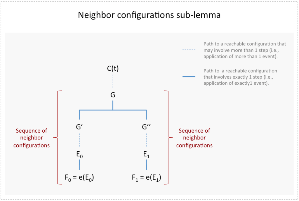
Neighbor configurations - FLP consensus impossibility

Suppose that for any two neighboring configurations $C_{0}$ and $C_{1} \in \mathcal{C},\ e(C_{0})$ and $e(C_{1})$ cannot have different valences. We’ve seen as part of Lemma A that $e(C_{0})$ and $e(C_{1})$ cannot have an empty set of decision values either. Furthermore, being elements of $\mathcal{D},$ they cannot be bivalent by the condition in Sub-lemma B.3. As a result, $e(C_{0})$ and $e(C_{1})$ must have the same valence.
In particular, since configurations $E_{0}$ and $G$ are linked by a sequence of neighbors, it must be that $e(E_{0})$ and $e(G)$ share the same valence. Given that $e(E_{0}) = F_{0}$ is 0-valent, it must be that $e(G)$ is 0-valent. By a similar argument, and using the sequence of neighbors linking $E_{1}$ and $G,$ we can also conclude that $e(G)$ is 1-valent. In other words, $e(G)$ is bivalent.
But $G \in \mathcal{C}$ and so $e(G) \in \mathcal{D}.$ A bivalent $e(G)$ contradicts the initial assumption that $\mathcal{D}$ has no bivalent configurations. Q.E.D.

Sub-lemma B.4 (“Commutativity property of schedules”): Suppose that from some configuration $C(t),$ schedules $\sigma_{1}$ and $\sigma_{2}$ lead to configurations $C_{1}(t')$ and $C_{2}(t'')$ respectively, for some $t', t'' > t.$ If the two sets of processors taking steps in $\sigma_{1}$ and $\sigma_{2}$ are disjoint, then the application of $\sigma_{2}$ to $C_{1}(t')$ and $\sigma_{1}$ to $C_{2}(t'')$ will result in the same configuration $C_{3}(t''')$ , for some $t''' >\ max(t',t'').$

Without loss of generality, suppose that the system’s processor set consists of two distinct processors $\{p_{1}, p_{2}\}.$ We will prove the sub-lemma for the simple case where the two schedules are disjoint singletons, i.e., $\sigma_{1} = \{e_{1} \equiv\ (p_{1}, m_{1})\}$ and $\sigma_{2} = \{e_{2} \equiv\ (p_{2}, m_{2})\}.$ The general case can be analyzed using the same logic.

Let $\sigma_{1}$ be initially applied to $C(t).$ The event $e_{1}$ corresponds to the receipt of message value $m_{1}$ by $p_{1}.$ Recall that the receive function deletes $(p_{1}, m_{1})$ from the message buffer $\mathcal{M}$ and then depending on $p_{1}$ ‘s internal state and on the message value $m_{1},$ $p_{1}$ enters a new internal state and sends a finite set of messages to other processors.
Let $C(t)\ \equiv$

$((x_{1}(t), s_{1}(t), c_{1}(t), y_{1}(t)),\ (x_{2}(t), s_{2}(t), c_{2}(t), y_{2}(t)),\ \mathcal{M}(t)).$

At $t',$ we can write:

$C_{1}(t') \equiv e_{1}(C(t)) =$

$((x_{1}(t'), s_{1}(t'), c_{1}(t'), y_{1}(t')),\ (x_{2}(t'), s_{2}(t'), c_{2}(t'), y_{2}(t')),$ $\mathcal{M}(t')) =$

$((x_{1}(t'), s_{1}(t'), c_{1}(t'), y_{1}(t')),\ (x_{2}(t), s_{2}(t), c_{2}(t), y_{2}(t)),$ $\mathcal{M}(t) - \{(p_{1}, m_{1})\}\ +\ A$ ),

where $A$ is a set of newly generated messages and processors pairs.

At $t''',$ we can write:

$C_{3}(t''') \equiv e_{2}(C_{1}(t')) =$

$((x_{1}(t'''), s_{1}(t'''), c_{1}(t'''), y_{1}(t''')),\ (x_{2}(t'''), s_{2}(t'''), c_{2}(t'''), y_{2}(t''')),$ $\mathcal{M}(t''')) =$

$((x_{1}(t'), s_{1}(t'), c_{1}(t'), y_{1}(t')),\ (x_{2}(t'''), s_{2}(t'''), c_{2}(t'''), y_{2}(t''')),$ $\mathcal{M}(t') - \{(p_{2}, m_{2})\}\ +\ B$ ),

where $B$ is a set of newly generated messages and processors pairs.

One can easily see that applying $\sigma_{2}$ to $C(t)$ and then applying $\sigma_{1}$ to the resulting configuration $C_{2}(t'')$ would yield the same configuration $C_{3}(t''').$

FLP consensus impossibility - Schedules commutativity

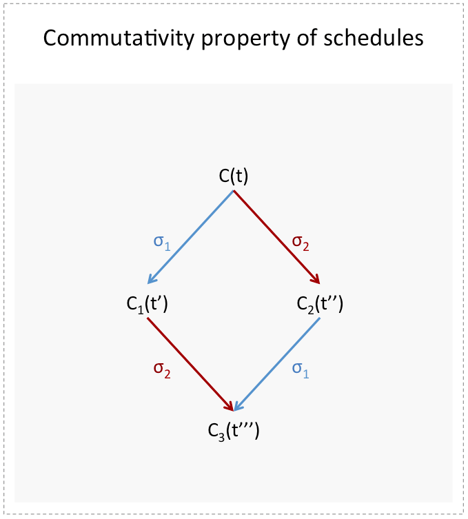
We are now in a position to prove Lemma B. Suppose that $\mathcal{D}$ has no bivalent configurations. By Sub-lemma B.3, there must exist two neighboring configurations $C_{0}, C_{1} \in \mathcal{C}$ such that $D_{0} \equiv e(C_{0})$ is 0-valent and $D_{1} \equiv e(C_{1})$ is 1-valent ( $e$ is the event $(p,m)$ ). By virtue of being neighbors, we can assume without loss of generality that $C_{1} = e'(C_{0})$ for some event $e' \equiv (p', m').$ We have two cases to consider:

Case $p \neq p'$ : We have $D_{1} = e(C_{1}) = e(e'(C_{0})).$ Since $p \neq p',$ then the two processors taking steps in $\sigma \equiv \{e\}$ and $\sigma' \equiv \{e'\}$ are disjoint. We can thus apply Sub-lemma B.4 to get $D_{1} = e'(e(C_{0})) = e'(D_{0}).$ This is not possible since a 1-valent configuration cannot be reached from a 0-valent one.
Case $p = p'$ : Consider an admissible run starting at $C_{0}$ and such that processor $p$ is the only faulty process and such that it is assumed to have crashed prior to starting the run. By the total correctness assumption, this admissible run must also be a deciding one. Let $\sigma$ be its corresponding schedule and let $A = \sigma(C_{0})$ be the resulting configuration. Clearly, the set $\{e, e'\} \equiv \{(p,m), (p,m')\}$ does not have any common processors with events included in $\sigma.$ We can thus invoke Sub-lemma B.4 as portrayed in the diagram below:

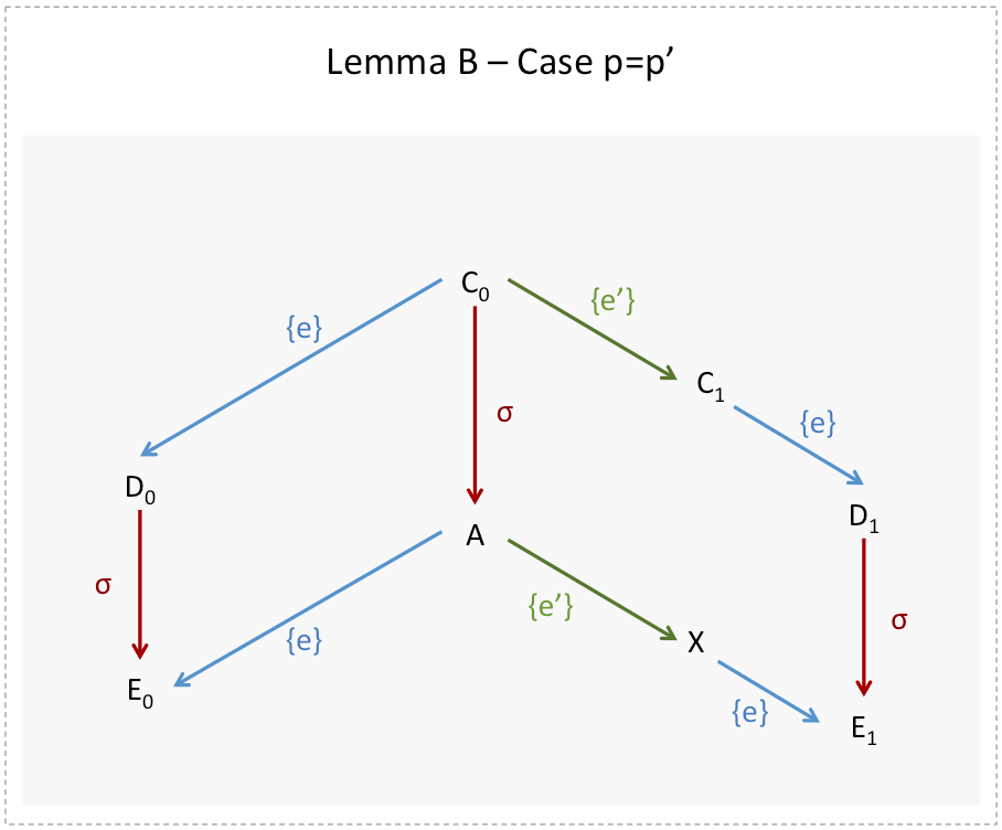
Since $D_{0}$ is 0-valent, it must be that $E_{0} \equiv \sigma(D_{0})$ is 0-valent too (we have previously shown as part of Lemma A that its decision set cannot be $\emptyset$ ). Similarly, since $D_{1}$ is 1-valent, so must be $E_{1}.$ Now note that $E_{0}$ and $E_{1}$ are both reachable from $A$ and have different valencies. $A$ must hence be bivalent. But $A$ is the outcome of a deciding run (by construction) and hence cannot be bivalent.

In both cases we reached a contradiction, demonstrating that $\mathcal{D}$ must contain at least one bivalent configuration.

In order to prove the FLP impossibility result, we now use Lemma A and Lemma B to build an admissible non-deciding run for any consensus protocol that is totally correct in spite of one fault. We first build a particular class of admissible runs as follows:

Maintain a queue of processors, originally in arbitrary order.
For any given configuration, let its associated message buffer be ordered according to the time the messages were sent, earliest first.
Define a stage to be a collection of one or more steps. A stage is completed when the first processor in the queue takes a step. In this step, the processor receives the earliest message destined to it in the message buffer, or $\emptyset$ if no messages are available. The processor is then moved to the back of the queue.

Note that this construction ensures that in any infinite sequence of such stages, every non-faulty processor (i.e., one that can take infinitely many steps) will receive every message sent to it. Such a run is hence admissible. We now derive a particular instance of a non-deciding run that belongs to this class of admissible runs. Let $C_{0}$ be any bivalent initial configuration (its existence is guaranteed by Lemma A), and repeat the following procedure for each bivalent configuration $C_{i},\ i \geq 0:$

Let $p$ be the processor heading the processors queue at the time corresponding to configuration $C_{i},$ and $m$ the earliest message value destined to $p$ in the message buffer (if there is no such message, then $m = \emptyset$ ). Let $e$ be the event $(p,m).$
Lemma B guarantees the existence of a bivalent configuration $C_{i+1}$ reachable from $C_{i}$ through the application of a schedule where $e$ is the last event applied.

The previous procedure is actually an infinite loop characterizing an admissible run with no decision ever reached. Q.E.D.

Before we wrap up this chapter, we stress one more time the importance of defining clearly the system model attributes. For example, it suffices to substitute the deterministic nature of the Termination criterion with its randomized counterpart for the FLP result to stop holding as was proven in [1].

5. References

[1] Michael Ben-Or. Another advantage of free choice: Completely asynchronous agreement protocols. ACM, 1983.

[2] Cynthia Dwork and Nancy Lynch. Consensus in the presence of partial synchrony. Journal of the Association for Computing Machinery, 35(2):288-323, April 1988.

[3] Michael J. Fischer, Nancy Lynch, and Michael Merritt. Easy impossibility proofs for distributed consensus problems. ACM, 1985.

[4] Michael J. Fischer, Nancy Lynch, and Michael S. Paterson. Impossibility of distributed consensus with one faulty process. Journal of the Association for Computing Machinery, 32(2):374-382, April 1985.

[5] Leslie Lamport, Robert Shostak, and Marchall Pease. The byzantine generals problem. ACM Transactions on programming Languages and Systems, 4(3):382-401,July 1982.

[6] M. pease, R. Shostak, and L. Lamport. Reaching agreement in the presence of faults. Journal of the Association for Computing Machinery, 27(2):228-234, April 1980.

Delfr

Consensus in distributed systems

1. Introduction

2. Distributed systems

3. The classical Byzantine Generals Problem

4. FLP impossibility result

5. References

No comments

Reply Cancel reply

Recent Posts

Categories

Delfr

Consensus in distributed systems

1. Introduction

2. Distributed systems

3. The classical Byzantine Generals Problem

4. FLP impossibility result

5. References

No comments

Reply Cancel reply

Stay in touch

Recent Posts

Categories